A Coordinated Electric System Interconnection Review—the utility’s deep-dive on technical and cost impacts of your project.
Challenge: Frequent false tripping using conventional electromechanical relays
Solution: SEL-487E integration with multi-terminal differential protection and dynamic inrush restraint
Result: 90% reduction in false trips, saving over $250,000 in downtime
The three operating regions you have to design to
| Device | Output vs voltage | Response | Best suited to | Main limitations |
|---|---|---|---|---|
| Mechanically switched capacitor or reactor | Proportional to voltage squared | Seconds; discrete steps; limited switching operations per day | Steady-state reactive supply, voltage profile, loss reduction | No dynamic capability; step voltage change on switching; capability collapses when most needed |
| Static var compensator | Capacitive branches proportional to voltage squared | A few cycles; continuously controllable | Continuous control where cost matters and deep voltage support is not the driver | Square-law capability loss; harmonic filters are part of the plant and interact with the network |
| STATCOM | Approximately proportional to voltage — constant current capability | One to two cycles closed loop; converter response faster still | Voltage stability margin, weak interconnections, fast disturbance recovery, flicker and unbalance compensation | Higher capital cost; converter losses; adds a converter and its control dynamics to the network |
| Synchronous condenser | Governed by machine capability and excitation | Excitation response in the hundreds of milliseconds; inherent inertial response instantaneous | System strength and inertia, short-circuit contribution, black start support | Rotating plant with maintenance and losses; slower controlled response than a converter |
| STATCOM with energy storage | Reactive as a STATCOM, plus real power within the storage rating | As STATCOM for reactive; real power limited by storage | Where a real power deficiency is part of the problem | Cost and complexity of the storage; different failure and maintenance profile |
| Stage | Keentel scope | Outcome |
|---|---|---|
| Screening | Series-compensation proximity, radial contingency review, UIF and short-circuit ratio screening, frequency scans | Early identification of which SSO types apply |
| Detailed studies | PSCAD/EMTDC EMT studies with vendor real-code models, impedance-based and frequency-scan analysis | Clear evidence of stability margins or risk |
| Model quality | EMT model review, benchmarking against positive-sequence models, model acceptance support | Models that system operators accept |
| Mitigation | Control retuning recommendations with vendors, SSDC and bypass logic requirements, protection and monitoring specifications | Practical, coordinated solutions |
| Interconnection support | SSR and SSO study reports for ISO and utility requirements, response to reviewer comments | Fewer delays in the interconnection process |
Resilience: designing CDUs to the facility Tier objective
Liquid cooling makes heat removal more critical, not less. Cold plates hold only seconds of thermal buffer. If TCS flow stops, processors throttle or shut down very quickly. Resilience design must therefore cover:
- Pump redundancy: N+1 pumps at minimum, with automatic changeover.
- CDU redundancy: N+1 CDUs on a common TCS header, or 2N CDUs serving A and B manifolds for fault-tolerant designs.
- Power to CDUs: dual-corded CDUs fed from A and B sources, with pumps and controls on UPS power so coolant keeps flowing through a utility failure and generator start. This is the liquid-cooling equivalent of continuous cooling.
- Facility water continuity: chilled water or condenser water must also continue, through thermal storage, UPS-backed pumps or a high enough FWS temperature that the TCS can coast on stored thermal mass for the transfer period.
- Concurrent maintainability: isolation valves so any CDU, pump, filter or manifold section can be serviced without stopping the others.
- Leak management: leak detection, drip trays, automatic isolation valves and procedures for fluid spills.
Electrical engineering considerations
CDUs and liquid-cooling plants are electrical loads with their own design requirements:
- Pump motors and VFDs. Large CDUs use variable-frequency drives on their pump motors. These introduce harmonic current that must be included in the facility's harmonic study and IEEE 519 evaluation.
- Critical mechanical load on UPS. Putting CDU pumps on UPS increases UPS and battery sizing. The mechanical UPS load must be included in redundancy and ride-through calculations.
- Feeder and protection design. Dual feeds, automatic transfer, selective coordination and arc-flash labelling apply to CDU power distribution just as they do to IT power.
- Generator transient response. CDU pumps restarting together after a transfer create motor inrush on the generators. Staged restarts and soft acceleration reduce the step load.
- Load dynamics. AI training loads can swing rapidly between high and low power. Cooling controls must track those swings without temperature overshoot, and electrical systems must handle both the IT and the cooling load changes.
Commissioning a liquid-cooled data hall
- Flush and clean the TCS piping and manifolds to the specified cleanliness, using high-purity flush water.
- Fill and vent with the specified coolant, verifying glycol concentration and chemistry.
- Pressure test for leaks at design and test pressures, including quick-disconnect fittings.
- Verify sensors and controls: flow meters, temperature sensors, pressure transmitters, leak detection and BMS points.
- Load test with heat load banks connected through the cold-plate interfaces or rack manifolds, across the operating range.
- Prove the heat balance on both loops at several load steps, and the approach temperature against the design.
- Test failure scenarios: pump failure, CDU failure, power transfer to generator, valve failure and loss of facility water, confirming temperatures stay within the IT vendor's limits.
How Keentel Engineering helps
Keentel Engineering supports data center owners, developers and EPCs with the electrical engineering that liquid-cooled facilities depend on, and coordinates with the mechanical engineer of record and cooling vendors on the integrated design.
Why Grid-Following Inverters Become Unstable Without a Grid Fault
October 21, 2026 | Blog
Part A — Weak-Grid Instability Without a Fault at a Glance
When engineers think about power system instability, they usually picture a short circuit: a lightning strike on a 345 kV line, a breaker failure, a cascade of trips. Grid-following inverters can become unstable in a quieter way. On a weak transmission system, a solar, wind or battery plant can oscillate or lose control during completely normal operation — a routine line outage for maintenance, a capacitor bank switching, a small change in power setpoint, a modest phase jump from a distant event, or simply an increase in output as the sun rises. No fault is required. The cause is the interaction between the inverter's own control loops and the impedance of the network it is connected to.
The mechanism in one paragraph
A grid-following inverter measures the voltage at its terminals, uses a phase-locked loop (PLL) to find that voltage's angle and frequency, and injects current aligned with it. On a strong grid, the injected current barely changes the measured voltage. On a weak grid, the network impedance is large, so every change in injected current changes the measured voltage — which changes the PLL output, which changes the current again. The inverter is no longer following an independent grid voltage; it is partly following itself. Whether that feedback loop settles or grows depends on network impedance, PLL and current-controller tuning, operating point, plant controller settings and the behavior of nearby converters.
What Keentel's analysis shows
Keentel Engineering ran a parameter scan of a grid-following inverter plant on a Thevenin grid at short-circuit ratios (SCR) from 1.2 to 5, with PLL bandwidths from 5 Hz to 40 Hz. The only disturbance was a 5° grid phase step — no fault, no voltage dip.
| SCR | 5 Hz | 10 Hz | 15 Hz | 20 Hz | 30 Hz | 40 Hz |
|---|---|---|---|---|---|---|
| 5 | Stable | Stable | Stable | Stable | Stable | Unstable |
| 4 | Stable | Stable | Stable | Stable | Stable | Unstable |
| 3 | Stable | Stable | Stable | Stable | Stable | Unstable |
| 2.5 | Stable | Stable | Stable | Stable | Stable | Unstable |
| 2 | Stable | Stable | Stable | Stable | Sustained oscillation | Unstable |
| 1.5 | Stable | Stable | Sustained oscillation | Sustained oscillation | Sustained oscillation | Unstable |
| 1.2 | Stable | Sustained oscillation | Sustained oscillation | Sustained oscillation | Unstable | Unstable |
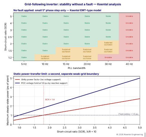
Figure 1. Top: stability map of the same plant at different SCR and PLL bandwidths, with no fault applied. Bottom: the separate static power-transfer limit of a grid-following plant as a function of SCR.
Three lessons from the map
- SCR matters, but it is not the whole story. At SCR 5, a 40 Hz PLL is still unstable in this model, because the instability at that bandwidth involves the current controller and output filter, not just grid strength.
- The stable region shrinks as the grid weakens. A tuning that works at SCR 3 may oscillate at SCR 1.5 — the SCR a plant might see during a planned outage.
- There are two different weak-grid limits. The dynamic (control interaction) limit in the top panel, and the static power-transfer limit in the bottom panel. Passing one does not guarantee passing the other.
A grid can remain free of faults and still present a challenging control environment for inverter-based resources. A single SCR value cannot describe every aspect of inverter-grid stability.
Part B — Why Can a Grid-Following Inverter Become Unstable Without a Grid Fault? An Engineering Guide for US Solar, Wind and Storage Interconnections
1. The changing US interconnection landscape
Inverter-based resources (IBRs) dominate the US interconnection queues. Solar, wind, battery storage and hybrid plants account for the overwhelming majority of new generating capacity requesting interconnection in ERCOT, MISO, SPP, PJM, CAISO, NYISO and ISO-NE, and in the vertically integrated utilities of the Southeast and West. Many of these plants are sited where land and resources are favorable — West Texas, the Great Plains, the desert Southwest, the Central Valley — often at the end of long 115 kV, 138 kV, 230 kV or 345 kV lines, far from large synchronous generators.
At the same time, synchronous generators that historically provided system strength are retiring. Coal units close, gas units cycle more, and nuclear units are not being replaced at the same rate. The result is that many points of interconnection (POIs) are becoming electrically weaker even as more inverter capacity connects to them.
NERC disturbance reports since 2016 have documented a long series of events in which inverter-based plants reduced output, tripped or oscillated in response to ordinary grid events. ERCOT has recorded oscillation events in West and South Texas associated with clusters of IBRs in low-strength areas. These are not exotic laboratory phenomena; they are now a routine consideration in US interconnection studies.
2. How a grid-following inverter works
2.1 The control chain
A grid-following inverter is a controlled current source. Its control chain has four main layers:
| Layer | Function | Typical bandwidth |
|---|---|---|
| Phase-locked loop (PLL) | Measures the angle and frequency of the voltage at the point of measurement | 5 to 50 Hz |
| Current control | Regulates d-axis (active) and q-axis (reactive) currents through the output filter | Several hundred hertz to over 1 kHz |
| Outer loops | DC-link voltage control, active power control, reactive power or voltage control | 1 to 20 Hz |
| Plant power controller (PPC) | Regulates POI voltage, reactive power, power factor and frequency response for the whole plant | 0.1 to 2 Hz, with communication delays of tens to hundreds of milliseconds |
2.2 The synchronous reference frame PLL
The most common PLL transforms measured three-phase voltages into a rotating dq frame and drives the q-axis component to zero with a proportional-integral (PI) controller:
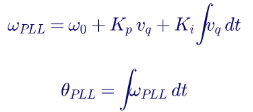
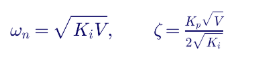
When locked, the d-axis aligns with the voltage vector, so d-axis current carries active power and q-axis current carries reactive power. The PLL's bandwidth — roughly its natural frequency — sets how quickly it tracks angle changes:
2.3 Why the measured voltage is not independent
The voltage at the point of measurement is the grid's Thevenin voltage plus the drop across the network impedance caused by the inverter's own current:

With a small Zgrid, VPCC is essentially Egrid, an independent reference. With a large Zgrid, VPCC depends strongly on Iinv. The PLL is then tracking a voltage that its own controller is moving. This closed loop through the network is the root of weak-grid control interaction.
3. Grid strength metrics
3.1 Short-circuit ratio
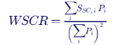
Consider three plants in one area:
| Plant | Rating | Short-circuit capacity at its POI | Single-plant SCR |
|---|---|---|---|
| A (wind) | 150 MW | 900 MVA | 6.0 |
| B (solar) | 200 MW | 750 MVA | 3.75 |
| C (storage) | 100 MW | 600 MVA | 6.0 |
Each plant appears comfortably strong on its own, but WSCR = (900 × 150 + 750 × 200 + 600 × 100) ÷ 450² = 1.70. Together, the three plants are in a weak-grid condition that none of their individual SCRs reveals. ERCOT uses WSCR in its screening and has identified areas where WSCR falls toward 1.5, the level at which detailed EMT studies and mitigation are expected.
Composite SCR (CSCR) is calculated from short-circuit capacity with all nearby IBR contributions removed, divided by the total IBR rating in the area. Both metrics capture the same reality: grid strength is shared.
3.4 Typical screening interpretation
| Metric value | Interpretation | Typical study response |
|---|---|---|
| Above 5 | Strong | Positive-sequence studies generally adequate |
| 3 to 5 | Moderate | Screening; EMT often required by transmission provider |
| 2 to 3 | Weak | EMT studies with vendor-specific models expected |
| 1.5 to 2 | Very weak | Special tuning, grid-forming capability or system strength additions likely |
| Below about 1.5 | Extremely weak | Interconnection may require network reinforcement or operating limits |
3.5 Why one SCR value is never enough
| Limitation | Why it matters |
|---|---|
| SCR is a single, fundamental-frequency number | Control interactions occur at frequencies from below 1 Hz to several hundred hertz, where network impedance is very different |
| SCR ignores X/R ratio | Resistive networks behave differently from purely inductive ones |
| SCR ignores shunt elements | Capacitors and filters create resonances and reduce effective strength |
| SCR ignores neighboring converters | Other IBRs, STATCOMs and HVDC links interact with the plant |
| SCR changes with system conditions | Outages, generator commitment and network topology shift SCR hour by hour |
| SCR says nothing about the inverter | The same SCR can be stable for one inverter design and unstable for another |
Keentel's stability map illustrates the last point clearly: at the same SCR, PLL bandwidth alone changes the outcome from stable to unstable.
4. Two different weak-grid limits
4.1 The static power-transfer limit
Even ignoring control dynamics, a weak network limits how much power a current source can push through it. For a plant at unity power factor connected through a Thevenin impedance, PCC voltage collapses as power increases. In Keentel's calculation with X/R = 10, the maximum steady-state power at unity power factor is approximately:

so a plant needs an SCR of about 1.8 to export its rating at unity power factor. With enough reactive support to hold PCC voltage at 1.0 pu, the limit rises to approximately the SCR itself:

| SCR | Max power at unity PF | Max power with voltage held at 1.0 pu |
|---|---|---|
| 5.0 | ≈ 2.77 pu | ≈ 5.0 pu |
| 3.0 | ≈ 1.66 pu | ≈ 3.0 pu |
| 2.0 | ≈ 1.11 pu | ≈ 2.0 pu |
| 1.5 | ≈ 0.83 pu | ≈ 1.5 pu |
| 1.2 | ≈ 0.66 pu | ≈ 1.2 pu |
| 1.0 | ≈ 0.55 pu | ≈ 1.0 pu |
Near these limits, the angle across the network approaches 90°, the voltage sensitivity to power becomes very high, and small disturbances can push the operating point past the nose of the PV curve. That is a loss of steady-state equilibrium — an instability that requires no fault.
4.2 Worked example: angle and voltage sensitivity
For a 100 MW plant at SCR 1.5 with X/R = 10, the network reactance on the plant base is about 0.66 pu. At rated output with voltage held at 1.0 pu:

At SCR 5, the same plant operates at about 11°. The voltage sensitivity to active power, dV/dP, is several times larger in the weak case. A PLL tracking angle and a voltage controller regulating magnitude both operate with much higher effective loop gain.
4.3 The dynamic (control interaction) limit
The second limit is dynamic: the closed loop formed by the PLL, current controller, voltage controller, plant controller and network impedance can become unstable at operating points well inside the static limit. This is the limit shown in the top panel of Figure 1, and it is the main subject of this guide.
5. Mechanisms of instability without a fault
| Mechanism | Typical frequency | What drives it |
|---|---|---|
| PLL–network interaction | About 2 to 30 Hz in the dq frame; appears as side-band frequencies around 60 Hz in phase quantities | High PLL bandwidth in a weak grid |
| Voltage control and plant controller interaction | About 0.5 to 5 Hz | High voltage control gains, PPC communication delays, several controllers regulating nearby buses |
| Current control and output filter interaction | Hundreds of hertz to kilohertz | Current controller bandwidth, sampling and PWM delay, LCL filter resonance, network capacitance |
| Converter-driven subsynchronous oscillation | About 5 to 55 Hz in phase quantities | Interaction with series-compensated lines or other converters |
| Harmonic resonance and harmonic instability | Above about 300 Hz | Converter output impedance negative damping near collector cable resonances |
| Converter-to-converter interaction | Wide range | Multiple plants, STATCOMs or HVDC links with overlapping bandwidths |
5.1 Frequency mapping between frames
Oscillations observed in the dq frame map to two side-band frequencies in phase quantities. An oscillation at fdq in the dq frame of a 60 Hz system appears at:

For example, a 15 Hz PLL-driven oscillation in the dq frame appears as components at about 45 Hz and 75 Hz in phase voltages and currents. Recognizing these side-bands in PMU, DFR or plant controller data is often the first clue that an event involves converter control interaction.
5.2 Triggers that are not faults
| Trigger | How it starts an oscillation |
|---|---|
| Planned transmission outage | Reduces SCR at the POI, moving the plant into a less stable region |
| Capacitor bank switching | Changes network impedance and introduces a voltage step |
| Morning ramp-up of solar output | Raises the operating point toward the static and dynamic limits |
| Setpoint changes from the plant controller or operator | Small step in power or voltage reference |
| Distant generator trip | Small phase and frequency step at the POI |
| Commissioning of a neighboring plant | Adds converter interaction and lowers WSCR |
| Firmware or parameter change | Alters control bandwidths |
6. Impedance-based stability analysis
6.1 The concept
Small-signal stability of an inverter connected to a grid can be analyzed by treating the inverter as a current source in parallel with an output impedance Zinv(s), and the grid as a voltage source behind Zgrid(s). The current flowing into the grid is:

The system is stable if the inverter is stable when connected to an ideal grid and the minor-loop gain Zgrid/Zinv satisfies the Nyquist criterion. In practice, engineers look for frequencies where:
- the magnitudes of Zinv and Zgrid cross, and
- the phase difference between them approaches or exceeds 180°, which happens when Zinv has a negative real part (negative damping).
6.2 Why the PLL creates negative resistance
At low frequencies, the PLL makes the inverter's q-axis impedance behave like a negative resistance whose magnitude grows with PLL bandwidth and active power output. Across a frequency band near the PLL bandwidth, the inverter therefore acts as an energy source for small perturbations. In a strong grid, the grid impedance is small and its magnitude does not cross the inverter impedance in that band. In a weak grid, the grid impedance magnitude rises and crosses in exactly the band where the inverter impedance is negatively damped. That is the frequency-domain view of the instability shown in Figure 1.
6.3 Practical frequency scanning
Engineers apply impedance analysis using frequency scans:
- Inverter scan: inject small perturbations at a series of frequencies into an EMT model of the inverter or plant (with the vendor's actual control code) and measure the response to obtain Zinv(f) or its dq matrix form.
- Network scan: obtain Zgrid(f) at the POI from an EMT or frequency-domain network model, including lines, cables, transformers, capacitor banks and filters.
- Stability assessment: apply Nyquist or generalized Nyquist criteria and identify frequencies and operating conditions with low margin.
- Confirm in time domain: verify critical cases with full EMT simulation.
Frequency scans are efficient for screening many network conditions and are increasingly requested by US transmission providers for low-strength interconnections.
7. Plant-level interactions
7.1 The plant controller
The plant power controller (PPC) regulates voltage or reactive power at the POI by sending setpoints to many inverters over a communication network. Its loop includes:
- measurement filters at the POI,
- PI or droop control,
- communication delays of tens to hundreds of milliseconds,
- inverter reactive current response,
- and the network's voltage sensitivity to reactive power.
The effective loop gain is proportional to the network's voltage sensitivity, approximately:

so the same PPC gain that is well damped at SCR 5 can be underdamped or unstable at SCR 1.5. Plant controller instability typically appears as slow voltage and reactive power oscillations, around 0.5 to 3 Hz.
7.2 Multiple plants regulating the same area
When several plants each regulate voltage at nearby buses with high gain and little droop, they can fight each other — one raising voltage while another lowers it — producing sustained oscillation. Coordinated voltage droop, appropriate gains and clearly assigned control responsibilities prevent this. The analysis must include all plants in the area, which is why WSCR-based screening and multi-plant EMT studies matter.
7.3 Collector system resonance
Large solar and wind plants contain long 34.5 kV collector cables whose capacitance resonates with transformer and network inductance, typically at several hundred hertz to a few kilohertz. If an inverter's output impedance is negatively damped near that resonance, harmonic instability can appear: growing distortion at a specific harmonic, often without any fundamental-frequency problem. These interactions require detailed collector models and vendor-specific inverter impedance data.
8. Model accuracy and validation
8.1 Why generic models are not enough
US planning studies use positive-sequence generic models — the WECC second-generation renewable models REGC, REEC and REPC — in PSS®E and PSLF. These are excellent for system-wide studies of active and reactive power response, voltage recovery and frequency response. They do not represent:
- the PLL and current controller in enough detail to capture fast control interaction,
- the converter's actual output impedance at frequencies above a few hertz,
- protection and fault-ride-through logic as implemented in firmware,
- or harmonics and resonances.
A positive-sequence study can show a plant as perfectly stable at an operating point where its actual control code would oscillate.
8.2 EMT models
Electromagnetic transient (EMT) models in PSCAD or similar tools simulate instantaneous three-phase waveforms with microsecond time steps, and vendor-specific models can include the inverter's real control code. NERC guidance recommends EMT models for IBRs in low-strength areas and identifies model quality expectations: correct initialization, representation of all relevant controls and protections, alignment with as-built settings and benchmarking against test data.
8.3 Model validation requirements
| Requirement | Role in weak-grid stability |
|---|---|
| NERC MOD-026 and MOD-027 (and successor model verification standards) | Verify voltage control, reactive power, active power and frequency response models against field data |
| IEEE 2800.2 test and verification procedures | Define how IEEE 2800 conformity, including dynamic performance, is verified through design evaluation, testing and commissioning |
| ISO/RTO and transmission owner model requirements | Many require vendor EMT models with specified quality checks before interconnection agreements |
| Post-commissioning validation | Compare recorded plant response during events with model results; update models when settings or firmware change |
8.4 Settings drift
A model is only as good as its parameter set. Inverter firmware updates, parameter changes during commissioning, plant controller retuning and the addition of new equipment can all invalidate a validated model. Change management — tracking every firmware version and parameter change and re-verifying stability when they change — is as important as the original study.
9. US requirements relevant to weak-grid stability
| Requirement | Relevance |
|---|---|
| IEEE Std 2800-2022 | Performance requirements for transmission-connected IBRs, including dynamic response, ride-through and stable operation for specified system conditions |
| NERC PRC-029 | Voltage and frequency ride-through for IBRs |
| NERC TPL-001 | Planning studies that must include IBR behavior and system strength conditions |
| NERC Reliability Guideline: Integrating IBRs into Low Short Circuit Strength Systems | Grid strength metrics, study methods and mitigation |
| NERC Reliability Guideline on EMT modeling of BPS-connected IBRs | When EMT models are needed and expected quality |
| FERC Order No. 2023 and related orders | Interconnection reform including model requirements and study processes |
| ERCOT, MISO, SPP, PJM, CAISO requirements | Weak grid screening (for example WSCR), EMT model submission and study requirements |
10. Mitigation options
| Mitigation | How it helps | Considerations |
|---|---|---|
| PLL and control retuning | Moves the plant into the stable region for the expected SCR range | Must not compromise ride-through, phase-jump response or frequency response |
| Vendor weak grid modes | Firmware designed for low SCR, often with adaptive gains | Requires model updates and validation |
| Plant controller tuning and droop | Damps slow voltage oscillations; prevents multi-plant fighting | Coordinate with transmission operator voltage schedules |
| Grid forming inverters | Voltage source behavior that does not rely on a conventional PLL; stable at very low SCR | Current limits during faults, protection coordination, emerging requirements |
| Synchronous condensers | Increase short circuit strength and inertia | Capital and operating cost; space |
| STATCOMs | Fast voltage support | Must be coordinated with IBR controls; can itself participate in interactions |
| Network reinforcement | Raises SCR permanently | Highest cost and longest lead time |
| Operating limits and outage dependent curtailment | Avoid unstable operating points | Lost energy; requires operator procedures |
| Passive or active damping of collector resonance | Reduces harmonic instability risk | Filter design, losses and harmonic compliance |
10.1 Worked example: how much synchronous condenser capacity?
Suppose a 300 MW solar plant has an SCR of 1.6 at its 230 kV POI under a critical N-1 outage, and EMT studies show the vendor's standard tuning requires an SCR of at least 2.0. The required short-circuit capacity is 2.0 × 300 = 600 MVA, compared with 1.6 × 300 = 480 MVA available. The deficit is 120 MVA of short-circuit contribution. A synchronous condenser contributes roughly its rating divided by its subtransient reactance through its step-up transformer:
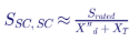

A 50 MVA condenser with X″d = 0.15 pu and a 0.10 pu step-up transformer contributes about 50 ÷ 0.25 = 200 MVA, more than enough in this simplified estimate. In practice, the contribution at the POI depends on where the condenser is connected, and the EMT study must confirm that the plant is stable with the condenser — and with the condenser out of service, if that is a credible condition.
11. A practical study workflow
- Screen grid strength with SCR, ESCR, WSCR or CSCR for normal and N-1 conditions, including planned outages and future projects.
- Request vendor models early: EMT model with exact firmware and parameters, plant controller model, inverter impedance data where available.
- Check model quality: initialization, flat runs, response to small steps, comparison with positive-sequence models.
- Build an adequate network model: enough of the transmission system, nearby IBRs, capacitor banks, series compensation and HVDC.
- Run small-disturbance cases: phase steps, voltage steps, power setpoint changes, capacitor switching and line switching across SCR conditions.
- Run large-disturbance cases: faults and ride-through, to confirm that tuning chosen for small-signal stability does not compromise fault response.
- Perform frequency scans where multiple converters or resonances are present.
- Identify and test mitigation: tuning, equipment, operating limits.
- Document settings and models that become part of the interconnection agreement.
- Validate after commissioning using high-resolution field data and update models as required.
12. Monitoring and event analysis
Even with careful studies, oscillations sometimes appear in operation. Early detection limits consequences:
| Data source | What it shows |
|---|---|
| PMUs at the POI and nearby substations | Oscillation frequency, magnitude and mode shape across the area |
| Plant DFRs and power quality meters | High-resolution waveforms showing side-band frequencies and harmonics |
| Inverter and plant controller logs | Control states, limits, setpoints and fault codes |
| SCADA trends | Slow oscillations and operating conditions |
| Oscillation detection tools at reliability coordinators | Automatic alarms for sustained oscillations |
When an oscillation is detected, operators can often stabilize the system quickly by reducing plant output, changing plant controller mode or restoring an outaged line, while engineers analyze the root cause.
13. Grid-following versus grid-forming: an engineering comparison
| Characteristic | Grid-following | Grid-forming |
|---|---|---|
| Synchronization | PLL tracks measured voltage | Internal voltage source with power synchronization or droop |
| Behavior at low SCR | Stability margin decreases; needs careful tuning | Typically stable at very low SCR |
| Behavior at very high SCR | Generally stable | Some designs need retuning for very strong grids |
| Fault current | Controlled current, typically 1.0 to 1.5 pu | Voltage-source behavior limited by current limits; transition between modes must be handled carefully |
| Inertia and fast response | Synthetic responses through control | Inherent fast response to voltage and frequency changes |
| Standards maturity | Well established | Requirements emerging in US ISO/RTO and NERC guidance |
Grid-forming capability is increasingly attractive for storage plants and hybrid projects in weak areas, but it is not a universal fix. Grid-forming plants must also be studied for their interaction with the network, protection and other converters.
14. Communicating results to transmission providers
A weak-grid stability study report that transmission providers can accept quickly typically includes:
- Grid strength assessment with all metrics and the contingencies considered.
- Model description, including firmware versions, parameter sets and model quality checks.
- Study cases, with disturbances, operating conditions and network configurations.
- Results, with plots and quantitative damping or oscillation metrics.
- Sensitivities, particularly to SCR, dispatch, PLL and PPC parameters.
- Mitigation and final settings.
- Commissioning and validation plan.
Clear, quantitative reporting reduces the cycles of comments and responses that can delay interconnection agreements.
15. Worked example: contingency SCR at a 230 kV POI
Grid strength must be checked for the conditions the plant will actually see, not only the all-lines-in-service case. Consider a 250 MW solar-plus-storage plant connected to a 230 kV switching station with three outgoing lines.
| Condition | Short-circuit capacity at POI | SCR (250 MW) | ESCR (with 40 Mvar filters) |
|---|---|---|---|
| All lines in service | 1,000 MVA | 4.0 | 3.84 |
| Line 1 out (strongest source) | 560 MVA | 2.24 | 2.08 |
| Line 2 out | 820 MVA | 3.28 | 3.12 |
| Line 1 out plus nearby combined cycle unit offline | 470 MVA | 1.88 | 1.72 |
| Line 1 and Line 2 out (N-2, maintenance plus forced outage) | 330 MVA | 1.32 | 1.16 |
The all-lines-in-service SCR of 4.0 suggests a moderately strong connection. But under the credible condition of the strongest line out with a nearby generator decommitted, ESCR falls to about 1.7 — inside the range where Keentel's stability map shows sustained oscillation for PLL bandwidths of 15 Hz and above. Under the N-2 condition, ESCR of 1.16 approaches the static limit of the plant at unity power factor (about 0.55 × 1.32 ≈ 0.73 pu of rating), so the plant could not export full power stably even with perfect controls.
The engineering conclusions are:
- The plant must be tuned and verified for ESCR down to about 1.7, not 4.0.
- An operating limit or automatic runback is needed for the N-2 condition, or that condition must be shown to be outside the planning criteria.
- The interconnection study must state which contingencies were considered, because the transmission provider will ask.
16. Worked example: plant controller loop gain versus SCR
A plant power controller regulates POI voltage with an integral gain Ki (pu
reactive power per pu voltage error per second). The voltage change caused by a reactive power change on the plant base is approximately:

so the effective integral loop gain seen by the controller is:

With a communication and processing delay Td, the loop is a delayed integrator. Its phase margin is approximately:

Suppose the controller has Ki = 20 pu/pu/s and Td = 150 ms (communication, measurement filtering and inverter response combined).
| SCR | Crossover ωc (rad/s) | Crossover frequency | Phase margin |
|---|---|---|---|
| 5.0 | 4.0 | 0.64 Hz | ≈ 56° |
| 3.0 | 6.7 | 1.06 Hz | ≈ 33° |
| 2.0 | 10.0 | 1.59 Hz | ≈ 4° |
| 1.5 | 13.3 | 2.12 Hz | Unstable |
The same gain gives a comfortable 56° phase margin at SCR 5, a marginal 4° at SCR 2, and instability at SCR 1.5 — a slow oscillation near 2 Hz, exactly the kind of event described in Case Study 1. The cure is not mysterious: scale the gain with expected SCR, add voltage droop (which reduces the effective integral action and shares regulation among plants), and reduce communication delay where possible. A simple sizing rule is to choose Ki so that the phase margin is at least 45° at the minimum credible SCR:
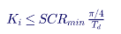
For SCRmin = 1.7 and Td = 0.15 s, Ki should not exceed about 8.9 pu/pu/s. This simplified calculation is a screening tool; the final gain must be verified with the vendor's plant controller model in EMT and positive-sequence simulation.
17. Worked example: how PLL bandwidth sets the vulnerable frequency band
A PLL tuned to bandwidth fPLL with damping ratio ζ has PI gains approximately

| PLL bandwidth | ωn (rad/s) | Kp (ζ=0.707, V = 1 pu) | Ki | Approximate phase-domain side-bands at risk |
|---|---|---|---|---|
| 5 Hz | 31 | 44 | 987 | 55 and 65 Hz |
| 10 Hz | 63 | 89 | 3,948 | 50 and 70 Hz |
| 20 Hz | 126 | 178 | 15,790 | 40 and 80 Hz |
| 30 Hz | 188 | 267 | 35,528 | 30 and 90 Hz |
The PLL introduces negative damping into the inverter's impedance around its own bandwidth, and the size of that negative damping scales with active power output. A 5 Hz PLL restricts the problem band to near-fundamental frequencies where the grid impedance is small and largely inductive. A 30 Hz PLL extends negative damping into a band where weak-grid impedance is large. That is why reducing PLL bandwidth is usually the first tuning lever.
The trade-off is that a slow PLL tracks phase jumps and frequency changes more slowly, which affects fault recovery, phase-jump ride-through and fast frequency response. IEEE 2800-2022 sets requirements for ride-through of phase-angle jumps and for performance during and after disturbances, so tuning must balance small-signal stability against large-disturbance performance. Keentel's practice is to scan PLL bandwidth across the full credible SCR range and confirm ride-through cases at the chosen setting, rather than optimizing for one condition.
18. Common misconceptions corrected
Weak-grid stability is often summarized in simplified ways that are directionally correct but incomplete. Keentel's review of the common explanations highlights the following points.
| Common statement | Engineering correction |
|---|---|
| "The instability happens without any disturbance." | In practice there is almost always a small trigger — a phase jump, line or capacitor switching, a setpoint change or a ramp in output. What is absent is a fault. The system was operating at a point with insufficient damping, and the small trigger revealed it. |
| "A weak grid is one with SCR below 3." | Thresholds of 3, 2 and 1.5 are screening guides. The relevant limit depends on the inverter design and settings, the X/R ratio, shunt elements and neighboring converters. Keentel's model showed instability at SCR 5 with an aggressive PLL. |
| "The PLL is the only cause." | The PLL is a common cause, but voltage controllers, plant controllers, current controllers, output filters and collector resonances can each drive instability at different frequencies. |
| "If the positive-sequence study is stable, the plant is stable." | Generic positive-sequence models do not represent the fast control dynamics that cause these interactions. EMT models with vendor control code are needed in weak areas. |
| "Higher control bandwidth is always better." | Faster controls improve response in strong grids but reduce stability margins in weak grids. Bandwidths must suit the grid. |
| "Waveforms in conceptual diagrams show how the plant will respond." | Illustrative waveforms explain the idea but are not measured data. Real oscillation frequency, damping and growth rate come only from validated models or field measurements. |
| "Adding a STATCOM always fixes weak grid problems." | A STATCOM supports voltage but does not add short circuit strength in the way a synchronous condenser does, and its own fast controls can participate in interactions. |
| "Grid forming inverters are immune." | Grid forming controls greatly improve low SCR performance but have their own interaction modes, current limiting behavior and protection implications that must be studied. |
19. Small-signal modeling in practice
19.1 State-space linearization
For research and detailed analysis, an inverter and network can be represented in state-space form and linearized around an operating p

The eigenvalues λ = σ ± jω of A show the frequency and damping of each mode. The damping ratio is:

Planning practice typically looks for damping ratios of at least 3 to 5% on all oscillatory modes under credible conditions, with some utilities specifying their own criteria. Participation factors identify which states — PLL, current controller, plant controller or network — dominate each mode, pointing directly to the most effective mitigation.
19.2 Limits of linear analysis
Linearized models are exact only for small perturbations. Real inverters include current limits, rate limits, mode switching (for example entering and leaving fault-ride-through logic) and protection. A mode that is lightly damped in a linear model may settle into a sustained oscillation bounded by a limiter, or a large disturbance may push the plant into a mode switch that a linear model cannot represent. Linear analysis is therefore a screening and insight tool; EMT simulation remains the reference.
19.3 Measuring damping from simulation or field data
When an oscillation is observed in an EMT run or in PMU data, the damping ratio can be estimated from successive peaks using the logarithmic decrement:

For example, if successive peaks of a 2 Hz reactive power oscillation are 12, 10.8 and 9.7 Mvar, δlog ≈ 0.105 and ζ ≈ 1.7% — well below a 5% criterion even though the oscillation is decaying. A decaying oscillation is not necessarily an acceptable one.
20. Data to request from inverter and plant controller vendors
| Item | Why it is needed |
|---|---|
| EMT model with actual control code and firmware version | Captures fast control interactions |
| Parameter file matching as-built settings | Model results depend on gains, limits and modes |
| Positive-sequence model and parameters | System wide planning and consistency checks |
| Inverter output impedance (dq frame) versus frequency and operating point | Enables impedance-based screening |
| Minimum SCR rating and weak grid mode description | Defines vendor stated capability |
| PLL type, bandwidth and adjustable range | Primary tuning lever |
| Plant controller structure, gains, droop, delays and communication architecture | Slow loop interaction analysis |
| Ride-through and protection settings | Ensures tuning does not compromise required performance |
| Model benchmarking reports against hardware or field tests | Confidence in model fidelity |
Requesting these items early in the interconnection process avoids study delays when the transmission provider identifies a low-strength condition.
20A. Commissioning and field verification in weak areas
Studies predict stability; commissioning proves it. In low-strength areas Keentel recommends a staged commissioning approach that tests the very controls most likely to interact with the network.
| Step | Test | Acceptance focus |
|---|---|---|
| 1 | Confirm as-built settings and firmware match the studied model | No undocumented parameter differences |
| 2 | Energize at reduced output (for example 25%) | Steady voltages and currents, no side-band components in DFR records |
| 3 | Small voltage reference steps in the plant controller (for example 1%) | Settling time and overshoot within the study envelope; damping ratio above the criterion |
| 4 | Small reactive power and active power setpoint steps | Response shape matches EMT and positive-sequence model results |
| 5 | Raise output in stages to rated power, repeating steps 3 and 4 | Damping does not degrade unacceptably with output |
| 6 | Capacitor bank or reactor switching near the POI, where operationally permitted | No sustained oscillation after switching |
| 7 | Record a baseline data set with high resolution DFR and PMU data | Reference for future model validation and event analysis |
Neutral-side CTs are often used for generator differential protection; terminal-side CTs are commonly used for directional power. The protection engineer must confirm which CT feeds the 32 element, that its polarity is correct for the chosen power convention and that its accuracy is appropriate.
16.1 Loss of potential
If a VT fuse blows or a VT circuit is opened, the measured voltage on one or more phases collapses, and the calculated three-phase power can be wrong in magnitude or sign. Reverse power elements should be supervised by loss-of-potential (LOP, device 60) logic, which blocks voltage-dependent functions when a VT problem is detected. Without this supervision, a VT fuse failure on a lightly loaded unit can cause a false reverse power trip.
17. Worked example 2: 100 MVA combustion turbine at 13.8 kV
Because motoring power is large, a pickup of half the motoring power — about 7% of MW rating, 6 MW — gives a large margin above measurement error:

With rated current of 4,184 A and full reactive output of about 60 Mvar, even a 0.5° angle error gives a measurement error of only about 0.5 MW, under 10% of the setting. The time delay is chosen from the manufacturer's allowable motoring duration and plant operating philosophy, typically 5 to 10 seconds.
The contrast with the steam unit is the core lesson: the same protection function needs completely different design attention depending on the prime mover. A combustion turbine 32 setting is easy to make secure; a condensing steam turbine 32 setting requires a measurement accuracy review.
18. Phase-angle compensation in numerical relays
Many numerical generator relays allow the engineer to enter a CT phase-angle correction. If the CT's phase displacement at low current is known from test data or the manufacturer's accuracy curves, the relay rotates the measured current phasor by the correction angle before calculating power:

The correction should be based on test data at the current levels seen during motoring, not at rated current, because CT phase errors are typically larger at low current. Overcompensation is as harmful as no compensation, so corrections should be verified during primary testing by comparing relay power with revenue metering at minimum stable load and high reactive output.
19. Motoring duration and turbine damage
Manufacturers often specify how long a unit can safely motor. For condensing steam turbines, allowable times depend on condenser vacuum, exhaust hood cooling sprays and blade design, and may range from several seconds to a few minutes. For units with non-condensing or back-pressure turbines, windage heating can be more severe. Factors that change allowable motoring time include:
- Condenser vacuum: poor vacuum increases windage losses and blade temperature.
- Exhaust hood sprays: spray water cools the last stages and extends allowable time, but can cause erosion if used excessively.
- Unit size: longer last-stage blades experience higher windage heating.
- Steam remaining in the turbine: extraction lines and reheaters can feed steam back into the turbine after a trip.
Reverse power time delays should be well inside the manufacturer's allowable motoring time, with margin for breaker failure clearing if the primary trip path fails.
20. Reading event records
When a generator trips on reverse power, the relay's event report and the plant's digital fault recorder (DFR) or sequence-of-events recorder (SER) show what happened. An engineer reviewing the event should check:
| Record | What it shows |
|---|---|
| Active power trace | Whether power fell gradually after a turbine trip, swung through zero during a system event, or reversed during synchronizing |
| Reactive power trace | Whether high reactive output may have affected measurement accuracy |
| Turbine trip and valve position contacts | Whether the trip was a planned sequential trip or a backup operation |
| Frequency and voltage | Whether a system disturbance caused a power swing |
| Element timing | Pickup time, delay, trip output and breaker opening |
| Breaker status | Whether the breaker opened correctly or breaker failure was needed |
Each step should be compared directly with simulation results using the same disturbance. Agreement in rise time, overshoot, settling time and oscillation frequency builds confidence that the model will predict behavior under conditions that cannot safely be tested in the field, such as low-SCR outages. Disagreement is an early warning that the model, the settings or the network representation needs correction — far better discovered at commissioning than during a summer peak with a key line out of service.
Commissioning tests in weak areas must be coordinated closely with the transmission operator. Test windows are often chosen when system strength is representative, and operators may require the ability to stop a test immediately if oscillations appear. A clear test plan with stop criteria, communication protocols and pre-agreed fallback settings is part of good engineering practice.
Ongoing performance monitoring
After commissioning, periodic review of plant event records against the validated model keeps the model honest. Keentel recommends reviewing any event in which the plant experiences a phase jump, voltage step or line switching above a defined threshold, and comparing recorded response with model playback. Gradual divergence can reveal component aging, undocumented setting changes or network changes that have altered system strength.
21. Key takeaways
- Instability does not require a fault. Normal operating changes can trigger control interaction in weak grids.
- The PLL makes the inverter follow a voltage it partly creates. That feedback through the network impedance is the root cause.
- There are two weak-grid limits: a static power-transfer limit and a dynamic control interaction limit.
- SCR is a screening tool, not a verdict. ESCR, WSCR, frequency-dependent impedance and inverter design all matter.
- Model accuracy is decisive. Generic positive-sequence models cannot show fast control interaction; validated vendor EMT models can.
- Mitigation has many forms: tuning, plant controller coordination, grid-forming technology, synchronous condensers and reinforcement.
22. How Keentel Engineering helps
Keentel Engineering performs grid strength, EMT and interconnection studies for solar, wind, storage and hybrid developers, independent power producers, utilities and transmission owners, from 4 kV to 765 kV.
| Stage | Keentel scope | Outcome |
|---|---|---|
| Grid strength screening | SCR, ESCR, WSCR and CSCR for normal, N-1 and planned outage conditions | Early identification of weak grid risk |
| EMT studies | PSCAD studies with vendor models: small-signal disturbances, faults, multi-plant interaction | Evidence of stable operation accepted by transmission providers |
| Frequency scans | Inverter and network impedance scans and Nyquist based assessment | Targeted mitigation with fewer time-domain cases |
| Plant controller tuning | PPC gain, droop and coordination studies | Damped voltage control and coordinated plants |
| Mitigation design | Vendor retuning, grid forming evaluation, synchronous condensers, STATCOM coordination | Practical, cost-effective solutions |
| Model validation | MOD-026/027 and IEEE 2800.2 support, event playback and model updates | Models that match field behavior |
| Interconnection support | Study reports, responses to transmission provider comments and commissioning support | Faster interconnection agreements |
Why clients choose Keentel Engineering
- Control-aware power system engineering: we understand the inverter's control loops as well as the network they connect to.
- EMT depth: detailed PSCAD modeling of plants, collector systems and transmission networks.
- Interconnection experience: practical knowledge of ERCOT, MISO, SPP, PJM, CAISO and utility study requirements.
- Vendor-neutral perspective: experience across inverter manufacturers and control architectures.
- Licensed professional engineering: a Florida-registered firm with offices in Tampa, Austin, Sacramento and Baltimore, supporting projects nationwide.
Interconnecting a solar, wind or storage project in a weak area? Talk to Keentel Engineering at (813) 389-7871, contact@keentelengineering.com, or book a 15-minute scoping call at calendly.com/keentel-engineering/15min.
Part C — Case Studies
The following are illustrative scenarios based on conditions typical of US IBR interconnections. They show how Keentel Engineering approaches weak-grid stability problems; site details are generalised and figures are rounded.
Case Study 1 — 200 MW solar plant at 138 kV: oscillation during a planned outage
Situation. A 200 MW solar plant connected at 138 kV operates normally for a year. During a planned outage of a nearby 138 kV line for maintenance, operators observe sustained 2 Hz oscillations in plant reactive power and POI voltage around midday. No fault occurred.
Analysis. Keentel's review shows that the SCR at the POI falls from about 3.2 with all lines in service to about 1.7 during the outage. PMU data show the oscillation in the plant controller's voltage loop. EMT studies with the vendor and PPC models reproduce the oscillation and confirm that the PPC voltage control gain, tuned for normal conditions, has very low damping at SCR 1.7.
Engineered solution. Keentel retunes the PPC voltage control with additional droop and reduced gain, verifies stability across the SCR range including outage conditions, and develops an operating procedure that limits plant output during specific planned outages until the new settings are commissioned.
Outcome. The plant operates stably through subsequent outages, and the transmission operator incorporates the outage-dependent operating guidance into its procedures.
Case Study 2 — 345 kV wind and storage cluster: WSCR and multi-plant interaction
Situation. A developer proposes a 250 MW battery plant near two existing wind farms at 345 kV. Each plant's individual SCR exceeds 3, but the transmission provider's WSCR screening for the area returns about 1.6.
Analysis. Keentel builds a multi-plant EMT model including both wind farms with their vendor models, the proposed battery and the surrounding 345 kV network. Small phase steps produce a poorly damped 12 Hz oscillation in the dq frame (visible as about 48 Hz and 72 Hz components in phase currents) involving the wind turbine converters and the battery's PLL. Frequency scans identify negative damping in the battery's impedance near the interaction frequency.
Engineered solution. Keentel evaluates the battery vendor's grid-forming option and a retuned grid-following option. The grid-forming configuration provides well-damped response across all studied conditions and improves damping for the existing wind farms.
Outcome. The battery is interconnected with grid-forming controls, the area's oscillation risk is reduced, and the study supports the transmission provider's broader weak-grid planning.
Case Study 3 — 150 MW solar plant at 115 kV: harmonic instability in the collector system
Situation. During commissioning of a 150 MW solar plant connected at 115 kV, voltage distortion at about the 23rd harmonic grows whenever output exceeds 60% of rating. Fundamental-frequency voltage and power are normal.
Analysis. Keentel's harmonic and EMT analysis shows a parallel resonance near 1.4 kHz formed by the long 34.5 kV collector cables and the main power transformer. The inverter's output impedance has negative damping near that frequency at higher output, driven by its current controller and PWM delay.
Engineered solution. Keentel works with the inverter vendor to enable active damping in the current controller and evaluates a small passive damping filter on the 34.5 kV bus as backup. Revised settings are verified with EMT simulation and field measurements.
Outcome. The harmonic growth disappears at all output levels, and voltage distortion at the POI meets IEEE 519 limits.
Part D — Technical FAQ: Weak-Grid Stability of Grid-Following Inverters
Yes. In weak grids, normal changes — outages, capacitor switching, setpoint changes or rising output — can trigger growing or sustained oscillations caused by interaction between inverter controls and network impedance.
An inverter that behaves as a controlled current source, synchronizing to the measured grid voltage with a phase-locked loop and injecting current aligned with that voltage.
In a weak grid, the inverter's own current changes the voltage the PLL measures. The PLL then partly tracks a voltage it is creating, forming a feedback loop through the network.
The short-circuit capacity at the POI, excluding the plant's own contribution, divided by the plant's rated power.
Effective short-circuit ratio subtracts shunt capacitor banks, filters and cable charging from the short-circuit capacity, because they reduce effective grid strength at the POI.
Weighted short-circuit ratio accounts for multiple IBR plants in one area by weighting each plant's short-circuit capacity by its rating. It reveals weak-grid conditions that single-plant SCRs hide.
SCR is a single fundamental-frequency number. It ignores X/R ratio, shunt elements, frequency-dependent impedance, neighboring converters, changing system conditions and the inverter's own design.
The static power-transfer limit, where PCC voltage collapses as power increases, and the dynamic control-interaction limit, where controls become unstable at operating points within the static limit.
In Keentel's simplified calculation with X/R = 10, about 1.8. With reactive support holding PCC voltage at 1.0 pu, the static limit falls to about 1.0. Dynamic limits are usually more restrictive.
From below 1 Hz (plant controller interaction) through several hertz to tens of hertz (PLL interaction) to hundreds of hertz or more (current control and resonance).
An oscillation at f in the dq frame of a 60 Hz system appears as side-bands at 60 − f and 60 + f Hz in phase voltages and currents.
A method that represents the inverter and grid as frequency-dependent impedances and applies a Nyquist criterion to their ratio, identifying frequencies where the inverter is negatively damped and the impedances cross.
They simplify PLL and current control and assume fundamental-frequency phasors, so they cannot capture fast control interactions or resonances that vendor EMT models reveal.
Yes. Plant controller voltage loops with high gain and communication delay can oscillate in weak grids, typically at 0.5 to 3 Hz, and multiple plants can fight each other.
Removing a line reduces SCR at the POI, which can move a plant from a stable to an unstable operating region without any fault.
They are generally much more stable at low SCR because they do not rely on a conventional PLL, but they still require studies for current limiting, protection and interaction with other equipment.
They increase short-circuit strength and add inertia, raising SCR and improving stability margins for nearby grid-following inverters.
Growth of distortion at a specific frequency, typically above 300 Hz, when an inverter's output impedance has negative damping near a network resonance such as collector cable capacitance resonating with transformer inductance.
IEEE 2800-2022 and IEEE 2800.2, NERC PRC-029, TPL-001 and model verification standards, NERC reliability guidelines on low short-circuit strength and EMT modeling, FERC Order No. 2023 and ISO/RTO-specific requirements.
Relying on a single SCR value and generic models, without studying outage conditions, multi-plant interaction and vendor-specific control behavior.
References and Further Reading
Links were current at publication (October 2026).
- IEEE Std 2800-2022, Standard for Interconnection and Interoperability of Inverter-Based Resources Interconnecting with Associated Transmission Electric Power Systems; IEEE P2800.2. IEEE.
- NERC Reliability Guideline, Integrating Inverter-Based Resources into Low Short Circuit Strength Systems. North American Electric Reliability Corporation.
- NERC Reliability Guideline, Electromagnetic Transient Modeling for BPS-Connected Inverter-Based Resources. North American Electric Reliability Corporation.
- NERC Reliability Standards PRC-029, TPL-001, MOD-026 and MOD-027; NERC disturbance reports on inverter-based resource performance. North American Electric Reliability Corporation.
- IEEE/CIGRE, Definition and Classification of Power System Stability — Revisited and Extended (2021). IEEE Transactions on Power Systems.
- J. Sun, Impedance-Based Stability Criterion for Grid-Connected Inverters. IEEE Transactions on Power Electronics.
- IEEE Std 519-2022, Standard for Harmonic Control in Electric Power Systems. IEEE.
- FERC Order No. 2023, Improvements to Generator Interconnection Procedures and Agreements. Federal Energy Regulatory Commission.
Disclaimer
This article is general technical information for educational purposes. It is not engineering advice for any specific project and does not create a professional relationship. The stability map and power-transfer limits come from Keentel Engineering's simplified single-plant models with illustrative parameters, not field data; actual stability limits depend on the specific inverter firmware, plant design, network and operating conditions and must be verified with validated vendor models. Project designs must follow current standards, transmission provider and ISO/RTO requirements and project-specific engineering analysis, sealed by a licensed professional engineer where required.
Case studies are illustrative scenarios based on typical project conditions, not records of specific client projects. Figures are rounded and indicative.
IEEE, NERC, FERC, ERCOT, WECC, PSS®E, PSLF, PSCAD™ and other names are the property of their respective owners. Keentel Engineering is not affiliated with or endorsed by these organisations or any software or equipment vendor.
| Office | Address | Phone |
|---|---|---|
| Head Office — Tampa | 400 N Ashley Dr STE #2600, Tampa FL 33602 | (813) 389-7871 |
| Austin | 5900 Balcones Drive STE 100, Austin TX 78731 | (512) 591-0752 |
| Sacramento | 1401 21st St Ste R, Sacramento CA 95811 | (916) 913-4524 |
| Baltimore | 306 W Redwood St STE 200, Baltimore MD 21201 | (410) 225-2181 |

About the Author:
Sandip "Sonny" R. Patel, P.E.
IEEE Senior Member · Founder & CEO, Keentel Engineering
In 1995, Sonny Patel earned his Electrical Engineering degree from the University of Illinois. But degrees don't build legacies — action does.
For three decades, he has worked the power industry from every side of the table: 16 years as a utility engineer at Exelon/Commonwealth Edison; generation leadership across hydroelectric, industrial steam turbine, and a 9 GW renewable fleet; NERC Regional Entity Senior Compliance Engineer and Audit Team Lead, auditing some of the nation's largest utilities; and testing and commissioning lead on equipment up to 765 kV — the very top of the North American grid.Utility. Generator. Regulator. Consultant. Few engineers have seen all four seats. Fewer still have sat in them.
His experience spans nuclear, hydro, conventional generation, renewables, oil and gas, mining — and today's data centers, where he is authoring a three-book series on data center design. He is a Licensed Professional Engineer in six states and a Licensed Electrical Contractor in Florida (Unlimited EC) — he doesn't just design the work; he's qualified to stand behind its execution.Today, as Founder and CEO of Keentel Engineering, Sonny leads a nationwide team of engineers delivering substation design, power system studies, NERC compliance, and commissioning — done right, coast to coast.Three decades. Every side of the table. One standard: accountable engineering.
Services

Let's Discuss Your Project
Let's book a call to discuss your electrical engineering project that we can help you with.
About the Author:
Sandip "Sonny" R. Patel, P.E.
IEEE Senior Member · Founder & CEO, Keentel Engineering
In 1995, Sonny Patel earned his Electrical Engineering degree from the University of Illinois. But degrees don't build legacies — action does.
For three decades, he has worked the power industry from every side of the table: 16 years as a utility engineer at Exelon/Commonwealth Edison; generation leadership across hydroelectric, industrial steam turbine, and a 9 GW renewable fleet; NERC Regional Entity Senior Compliance Engineer and Audit Team Lead, auditing some of the nation's largest utilities; and testing and commissioning lead on equipment up to 765 kV — the very top of the North American grid.
Utility. Generator. Regulator. Consultant. Few engineers have seen all four seats. Fewer still have sat in them.
His experience spans nuclear, hydro, conventional generation, renewables, oil and gas, mining — and today's data centers, where he is authoring a three-book series on data center design. He is a Licensed Professional Engineer in six states and a Licensed Electrical Contractor in Florida (Unlimited EC) — he doesn't just design the work; he's qualified to stand behind its execution.
Today, as Founder and CEO of Keentel Engineering, Sonny leads a nationwide team of engineers delivering substation design, power system studies, NERC compliance, and commissioning — done right, coast to coast.Three decades. Every side of the table. One standard: accountable engineering.
Leave a Comment
Thank you for contacting us.
We will get back to you as soon as possible.
We will get back to you as soon as possible.
Oops, there was an error sending your message.
Please try again later.
Please try again later.
Related Posts
By SANDIP R PATEL
•
October 20, 2026
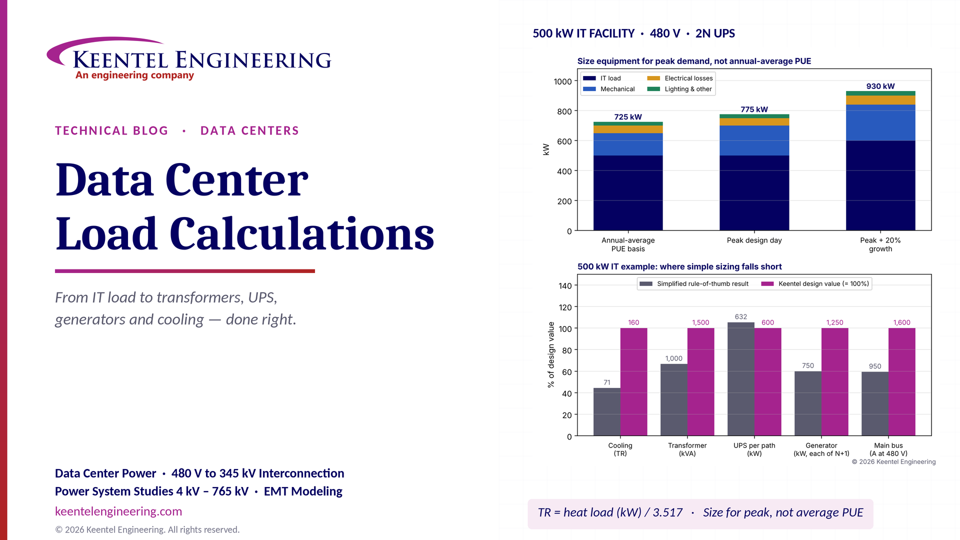
Learn data center electrical load calculations, including IT demand, PUE, UPS and generator sizing, cooling loads, redundancy, and worked US examples.
By SANDIP R PATEL
•
October 20, 2026
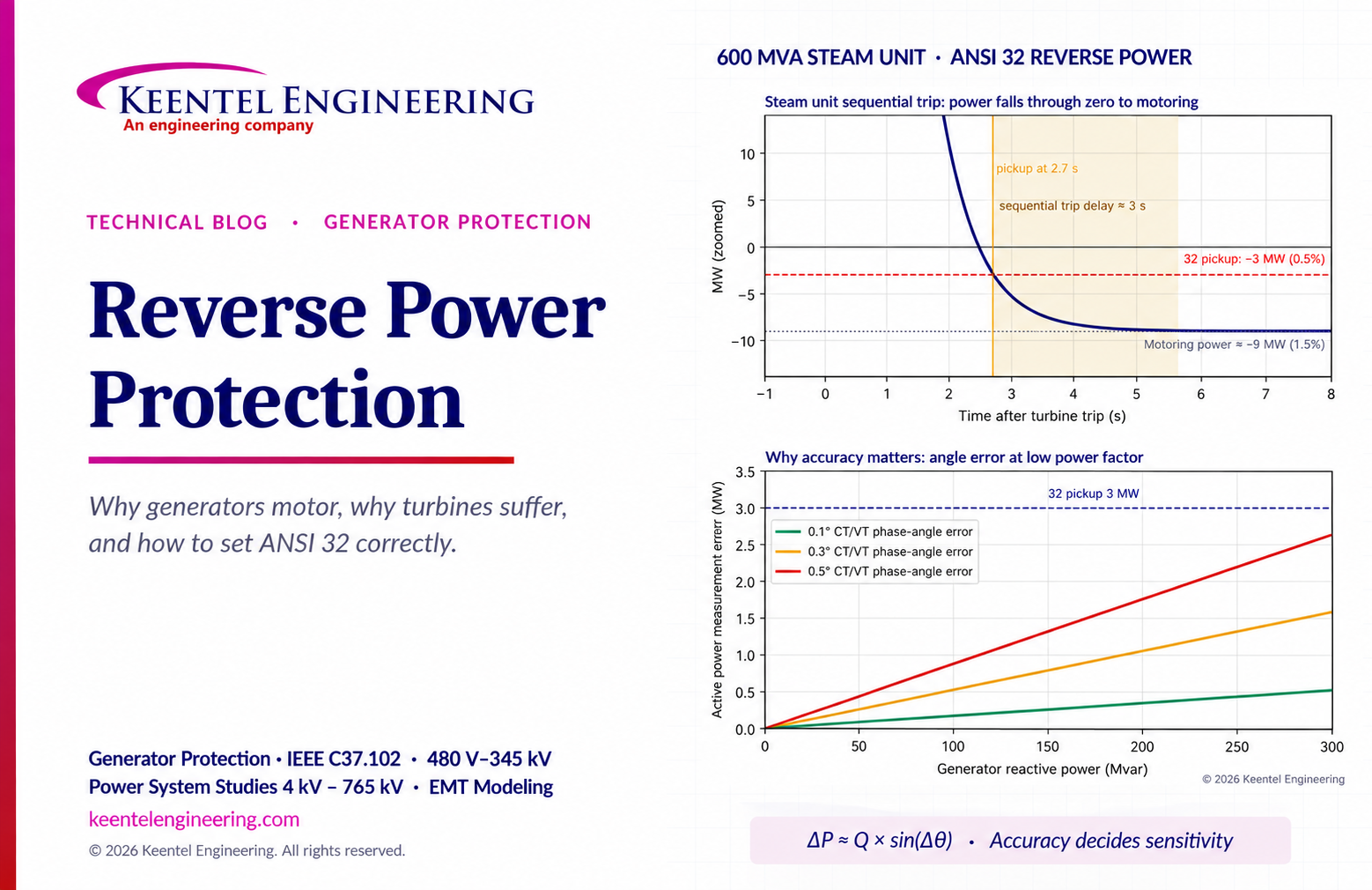
Learn reverse power protection (ANSI 32), generator motoring, relay pickup settings, time delays, sequential tripping and testing for US power plants.
Copy
By Team 2 Dexora
•
October 20, 2026
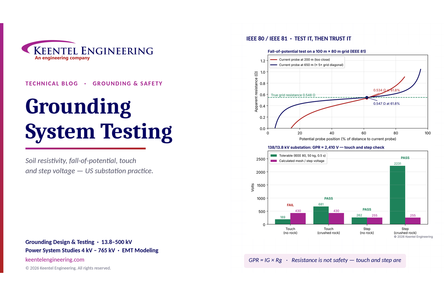
Explore grounding system testing with Keentel Engineering. Learn IEEE 80/81 methods, soil resistivity, ground resistance, and touch and step voltage safety.
By SANDIP R PATEL
•
October 13, 2026
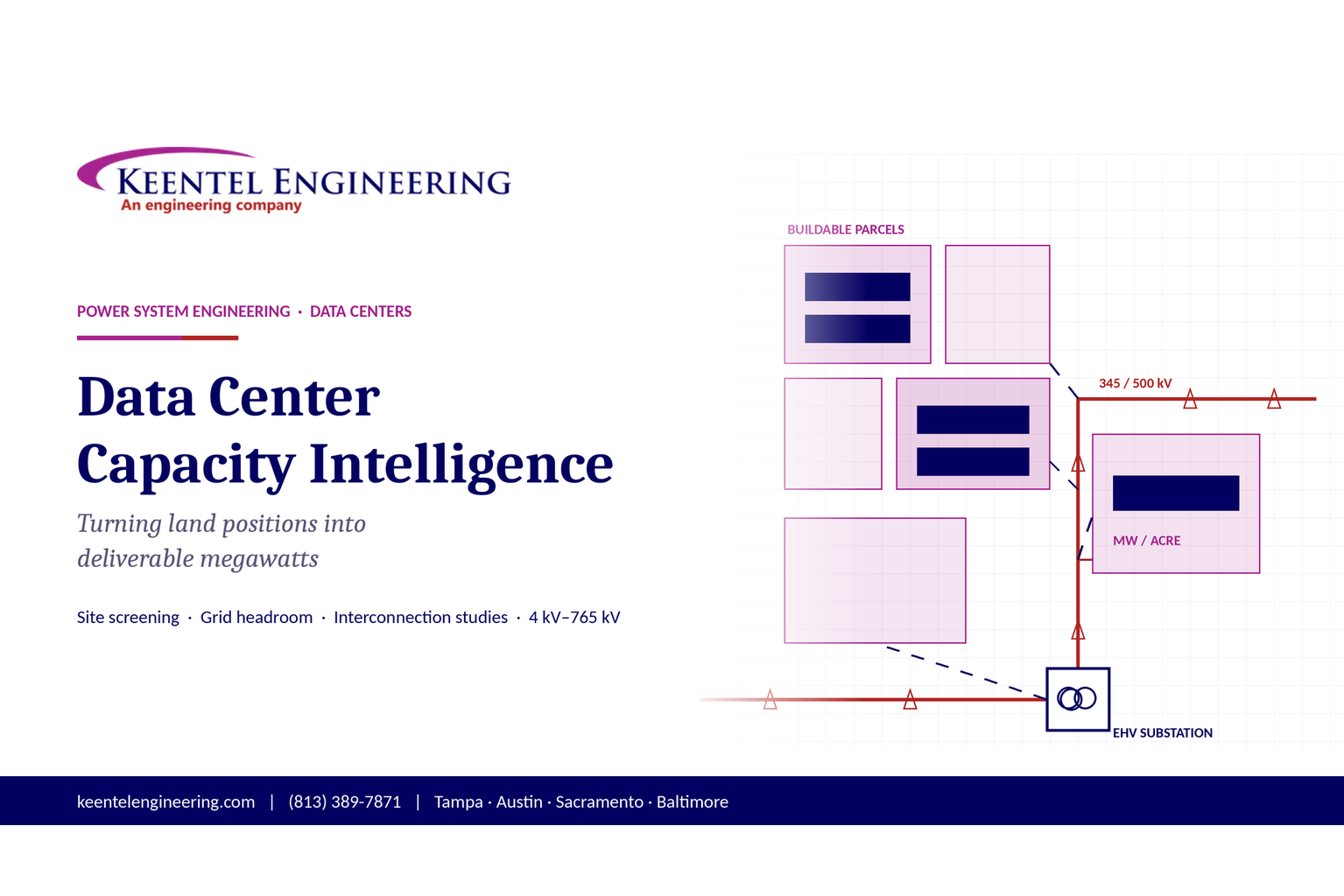
Plan data center capacity with land screening, MW-per-acre estimates, grid power availability and interconnection feasibility studies from Keentel Engineering.
By SANDIP R PATEL
•
October 11, 2026
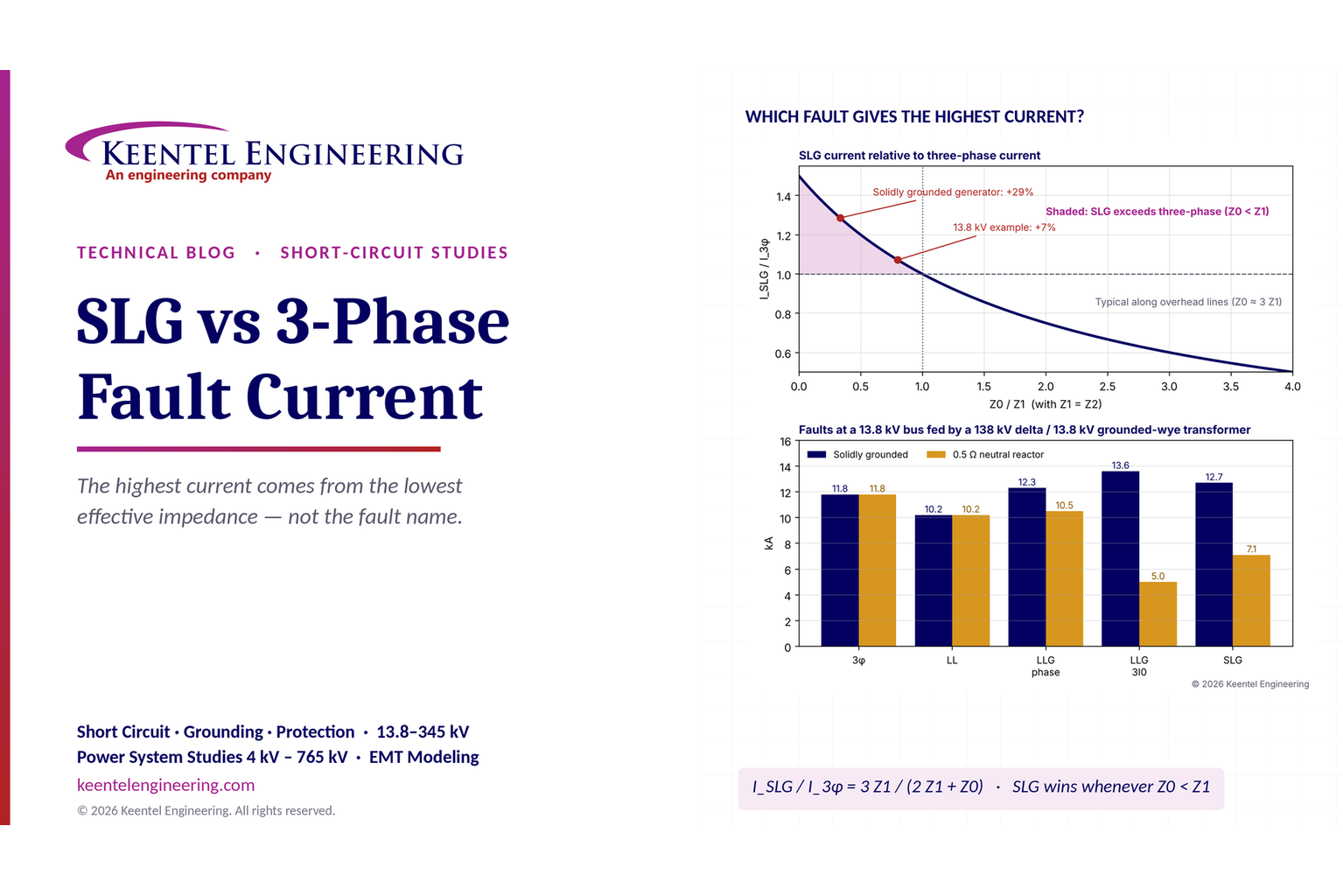
Learn which fault produces the highest current at a bus, why SLG faults can exceed three-phase faults, and how symmetrical components determine fault duty.
By SANDIP R PATEL
•
October 11, 2026
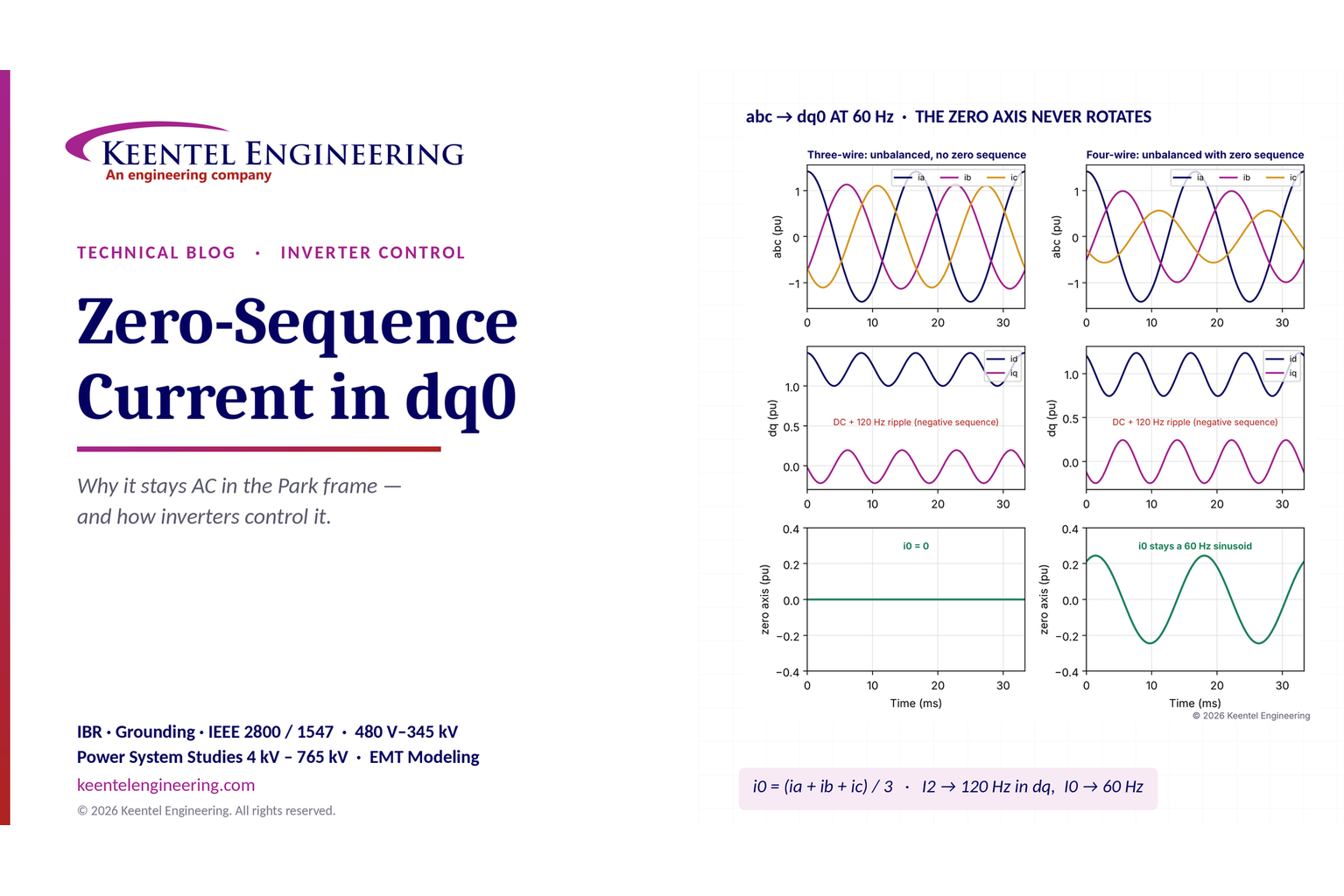
Learn why zero-sequence current pulsates in the dq0 frame, how Park's transformation works, and how inverter controls handle unbalance and ground faults.
By SANDIP R PATEL
•
October 11, 2026
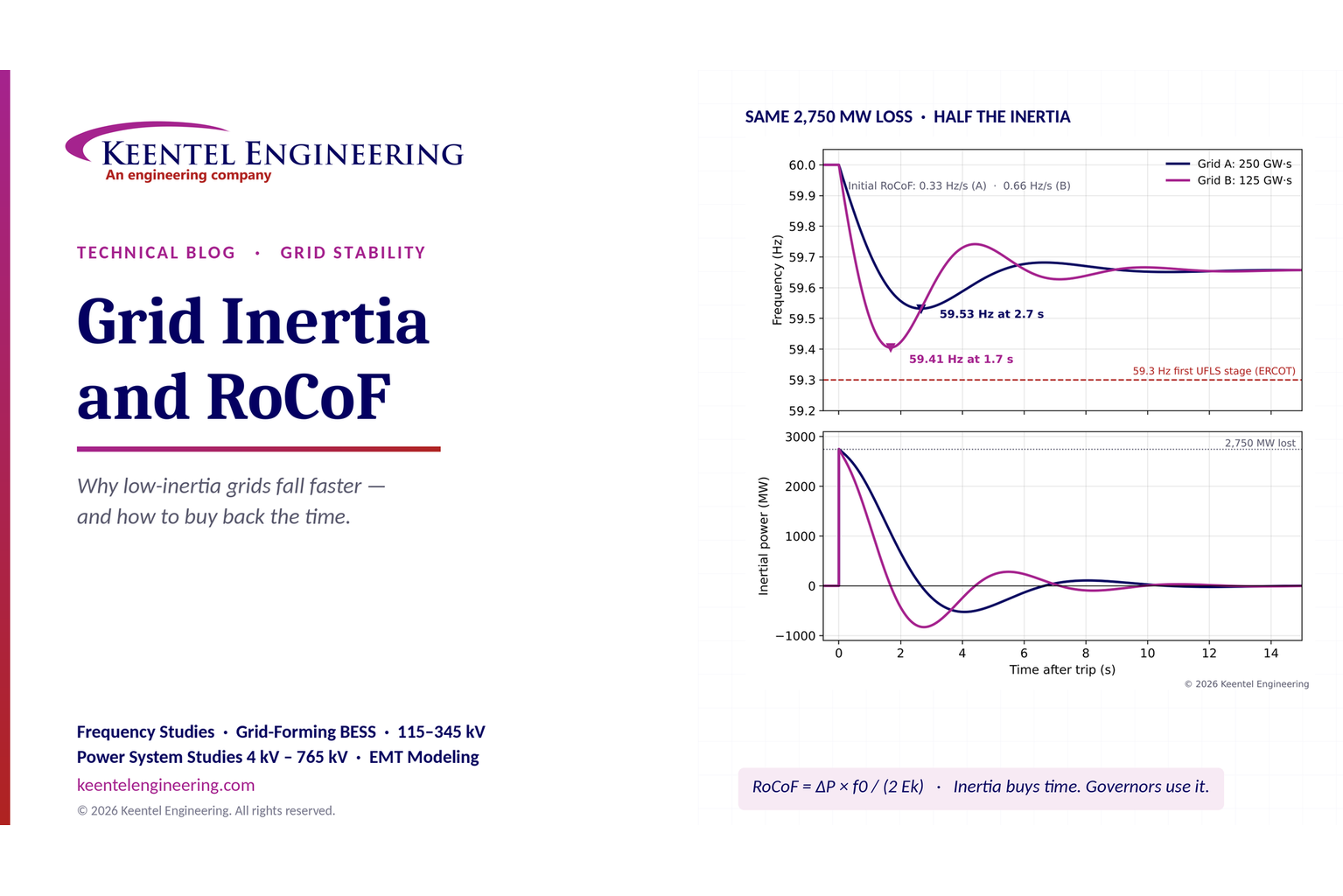
Explore grid inertia, RoCoF and frequency response, with swing equation calculations, frequency nadir analysis and US power system simulation examples.
By SANDIP R PATEL
•
October 11, 2026
Learn transient stability analysis, swing equation, equal-area criterion and critical clearing time with a 345 kV worked example and NERC TPL-001 guidance.
By SANDIP R PATEL
•
October 11, 2026
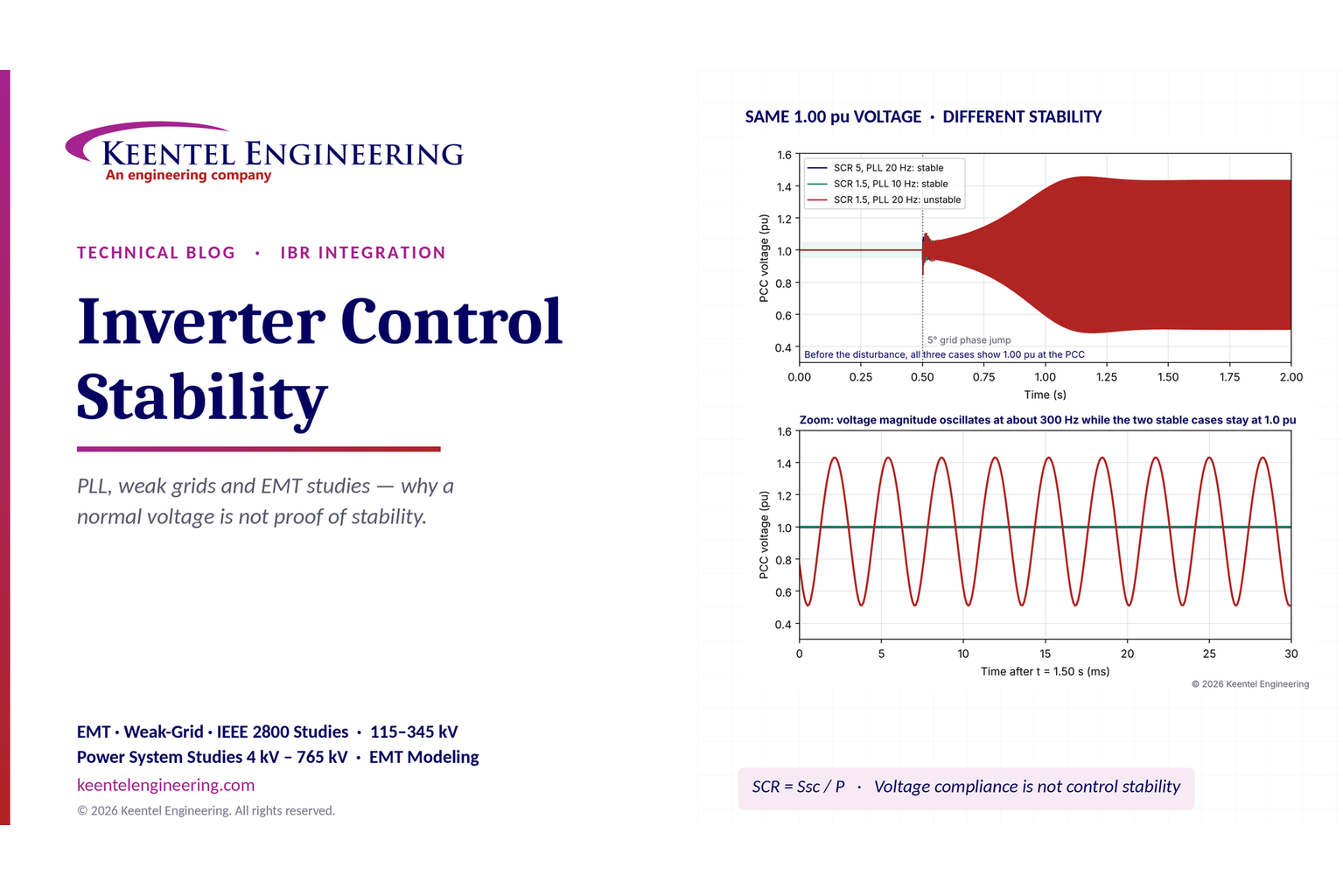
Learn why inverter controls become unstable in weak grids, how PLL bandwidth and SCR affect stability, and how PSCAD EMT studies identify and mitigate oscillations.