A Coordinated Electric System Interconnection Review—the utility’s deep-dive on technical and cost impacts of your project.
Challenge: Frequent false tripping using conventional electromechanical relays
Solution: SEL-487E integration with multi-terminal differential protection and dynamic inrush restraint
Result: 90% reduction in false trips, saving over $250,000 in downtime
The three operating regions you have to design to
| Device | Output vs voltage | Response | Best suited to | Main limitations |
|---|---|---|---|---|
| Mechanically switched capacitor or reactor | Proportional to voltage squared | Seconds; discrete steps; limited switching operations per day | Steady-state reactive supply, voltage profile, loss reduction | No dynamic capability; step voltage change on switching; capability collapses when most needed |
| Static var compensator | Capacitive branches proportional to voltage squared | A few cycles; continuously controllable | Continuous control where cost matters and deep voltage support is not the driver | Square-law capability loss; harmonic filters are part of the plant and interact with the network |
| STATCOM | Approximately proportional to voltage — constant current capability | One to two cycles closed loop; converter response faster still | Voltage stability margin, weak interconnections, fast disturbance recovery, flicker and unbalance compensation | Higher capital cost; converter losses; adds a converter and its control dynamics to the network |
| Synchronous condenser | Governed by machine capability and excitation | Excitation response in the hundreds of milliseconds; inherent inertial response instantaneous | System strength and inertia, short-circuit contribution, black start support | Rotating plant with maintenance and losses; slower controlled response than a converter |
| STATCOM with energy storage | Reactive as a STATCOM, plus real power within the storage rating | As STATCOM for reactive; real power limited by storage | Where a real power deficiency is part of the problem | Cost and complexity of the storage; different failure and maintenance profile |
| Stage | Keentel scope | Outcome |
|---|---|---|
| Screening | Series-compensation proximity, radial contingency review, UIF and short-circuit ratio screening, frequency scans | Early identification of which SSO types apply |
| Detailed studies | PSCAD/EMTDC EMT studies with vendor real-code models, impedance-based and frequency-scan analysis | Clear evidence of stability margins or risk |
| Model quality | EMT model review, benchmarking against positive-sequence models, model acceptance support | Models that system operators accept |
| Mitigation | Control retuning recommendations with vendors, SSDC and bypass logic requirements, protection and monitoring specifications | Practical, coordinated solutions |
| Interconnection support | SSR and SSO study reports for ISO and utility requirements, response to reviewer comments | Fewer delays in the interconnection process |
Resilience: designing CDUs to the facility Tier objective
Liquid cooling makes heat removal more critical, not less. Cold plates hold only seconds of thermal buffer. If TCS flow stops, processors throttle or shut down very quickly. Resilience design must therefore cover:
- Pump redundancy: N+1 pumps at minimum, with automatic changeover.
- CDU redundancy: N+1 CDUs on a common TCS header, or 2N CDUs serving A and B manifolds for fault-tolerant designs.
- Power to CDUs: dual-corded CDUs fed from A and B sources, with pumps and controls on UPS power so coolant keeps flowing through a utility failure and generator start. This is the liquid-cooling equivalent of continuous cooling.
- Facility water continuity: chilled water or condenser water must also continue, through thermal storage, UPS-backed pumps or a high enough FWS temperature that the TCS can coast on stored thermal mass for the transfer period.
- Concurrent maintainability: isolation valves so any CDU, pump, filter or manifold section can be serviced without stopping the others.
- Leak management: leak detection, drip trays, automatic isolation valves and procedures for fluid spills.
Electrical engineering considerations
CDUs and liquid-cooling plants are electrical loads with their own design requirements:
- Pump motors and VFDs. Large CDUs use variable-frequency drives on their pump motors. These introduce harmonic current that must be included in the facility's harmonic study and IEEE 519 evaluation.
- Critical mechanical load on UPS. Putting CDU pumps on UPS increases UPS and battery sizing. The mechanical UPS load must be included in redundancy and ride-through calculations.
- Feeder and protection design. Dual feeds, automatic transfer, selective coordination and arc-flash labelling apply to CDU power distribution just as they do to IT power.
- Generator transient response. CDU pumps restarting together after a transfer create motor inrush on the generators. Staged restarts and soft acceleration reduce the step load.
- Load dynamics. AI training loads can swing rapidly between high and low power. Cooling controls must track those swings without temperature overshoot, and electrical systems must handle both the IT and the cooling load changes.
Commissioning a liquid-cooled data hall
- Flush and clean the TCS piping and manifolds to the specified cleanliness, using high-purity flush water.
- Fill and vent with the specified coolant, verifying glycol concentration and chemistry.
- Pressure test for leaks at design and test pressures, including quick-disconnect fittings.
- Verify sensors and controls: flow meters, temperature sensors, pressure transmitters, leak detection and BMS points.
- Load test with heat load banks connected through the cold-plate interfaces or rack manifolds, across the operating range.
- Prove the heat balance on both loops at several load steps, and the approach temperature against the design.
- Test failure scenarios: pump failure, CDU failure, power transfer to generator, valve failure and loss of facility water, confirming temperatures stay within the IT vendor's limits.
How Keentel Engineering helps
Keentel Engineering supports data center owners, developers and EPCs with the electrical engineering that liquid-cooled facilities depend on, and coordinates with the mechanical engineer of record and cooling vendors on the integrated design.
Ferranti Effect in Transmission Lines: Causes and Mitigation
October 21, 2026 | Blog
Part A — The Ferranti Effect at a Glance
Energize a long extra-high-voltage transmission line from one end and leave the far end open, and the voltage at the open end is higher than the voltage at the source. Nothing has failed. No load is connected. The line itself, through its own distributed capacitance and series inductance, creates the rise. This is the Ferranti effect, first observed in the 1880s on a cable feeding London from the Deptford power station, and it remains one of the first constraints an engineer checks when energizing, restoring, or lightly loading a long 230 kV, 345 kV, 500 kV or 765 kV line.
The mechanism in one paragraph
A transmission line has capacitance distributed along its length. Under no load or light load, that capacitance draws charging current, which leads the voltage by 90°. The charging current flows through the line's series inductance, and the voltage drop across an inductance carrying a leading current is a voltage rise. The rise accumulates toward the open end, where all of the downstream charging has been supplied. The longer the line, and the higher the frequency, the larger the rise.
What Keentel's long-line model shows
Keentel Engineering modeled a representative 345 kV line with twin-bundled conductors (R = 0.030 Ω/km, X = 0.370 Ω/km and B = 4.5 µS/km at 60 Hz) using exact distributed-parameter equations, cascaded pi sections and an EMT traveling-wave model.
| Case: 217-mile (350 km) line, receiving end open | Receiving-end voltage rise |
|---|---|
| Same line at 50 Hz, stiff source (reference) | 7.5% |
| 60 Hz, stiff source, exact long-line solution | 11.1% |
| 60 Hz, single nominal pi section | 11.4% (overestimates) |
| 60 Hz, ten cascaded pi sections | 11.1% |
| 60 Hz, 10,000 MVA source, rise relative to source EMF | 13.4% |
| 60 Hz, 5,000 MVA source, rise relative to source EMF | 15.8% |
| 60 Hz, 50% shunt reactor compensation | 5.4% |
| 60 Hz, 70% shunt reactor compensation | 3.2% |
| Energization at a voltage peak (EMT, 10,000 MVA source, no mitigation) | Transient peak ≈ 2.2 pu |
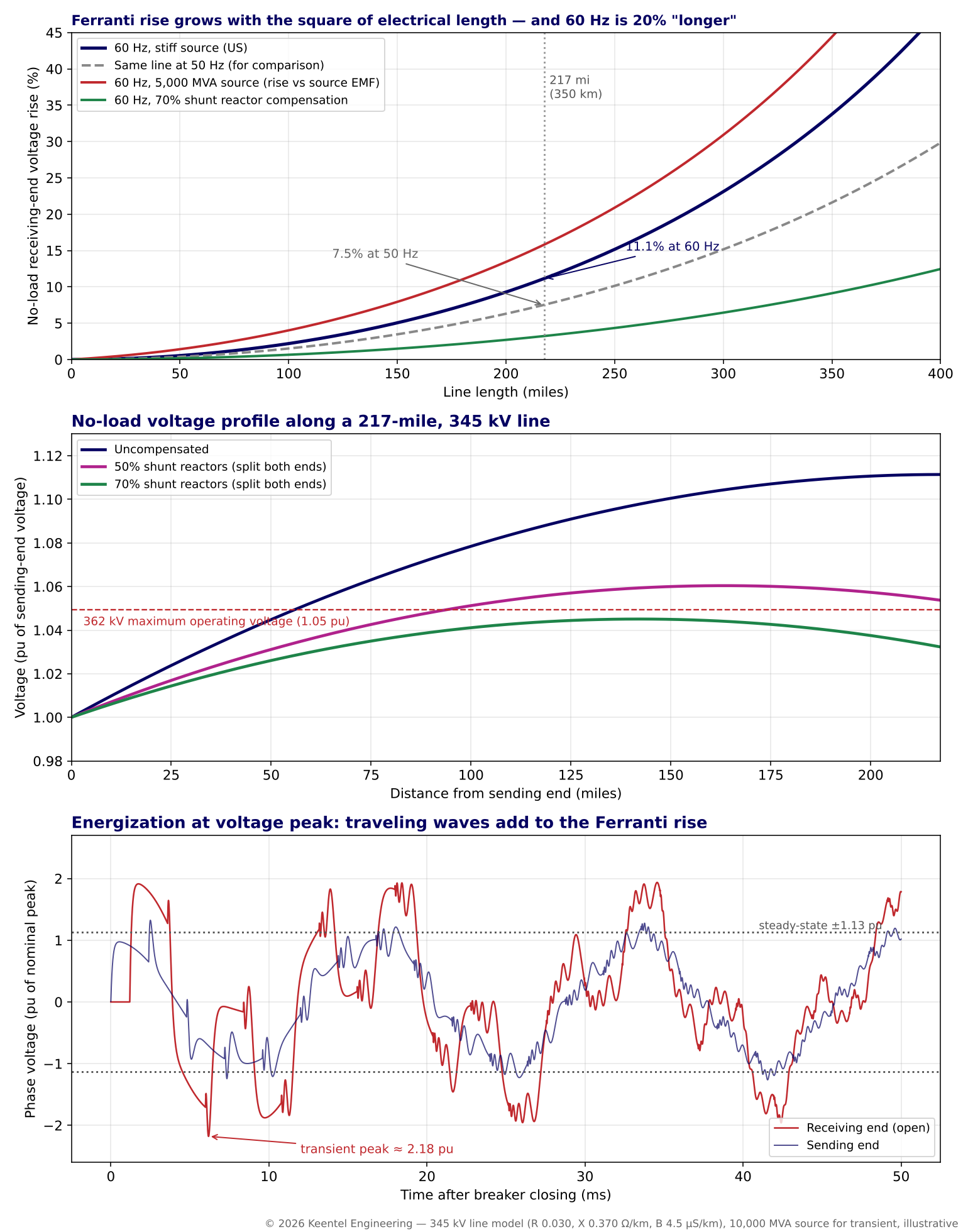
Figure 1. Top: no-load receiving-end voltage rise versus line length. Middle: voltage profile along a 217-mile, 345 kV line with and without shunt reactors. Bottom: EMT waveform of energization at a voltage peak, showing traveling-wave overvoltage on top of the steady-state Ferranti rise.
Four lessons from the model
- US 60 Hz lines see a larger Ferranti rise than the same line at 50 Hz. Electrical length scales with frequency, and the rise scales roughly with the square of electrical length. A line that rises 7.5% at 50 Hz rises about 11% at 60 Hz — enough to push a 345 kV line beyond its 362 kV maximum operating voltage.
- The source matters. Line charging current flowing through the source impedance raises the sending-end voltage too. With a weaker source, the open-end voltage relative to the system's internal voltage is substantially higher than the line-only calculation suggests.
- For steady-state rise, every reasonable line model agrees. Frequency-dependent, Bergeron and multi-section pi models all predict essentially the same 60 Hz no-load voltage. Model choice matters for transients, not for the steady-state Ferranti calculation.
- The steady-state rise is only the starting point. Switching transients during energization can more than double the instantaneous voltage at the open end, so insulation coordination, surge arresters and switching practice must be checked together with the steady-state rise.
Engineering review of a typical published simulation
Keentel reviewed a published comparison of a 50 Hz, 350 km double-circuit EHV line simulated with frequency-dependent, Bergeron and pi-section models. The reported results were 7.50%, 7.53% and 7.63% receiving-end voltage rise respectively.
| Published statement | Keentel's check |
|---|---|
| All three models predict about 7.5% rise on a 350 km line at 50 Hz. | Confirmed. Keentel's exact long-line calculation for comparable 50 Hz parameters gives 7.52%. |
| The pi section model gives the highest rise | Consistent with theory. A lumped pi representation slightly overestimates the rise unless the line is divided into enough sections; Keentel's single-section 60 Hz case overestimates by 0.2 percentage points. |
| Voltage rise (%) = (Vr − Vs) ÷ Vs × 100 | Correct definition, but it measures rise relative to the sending-end bus only. Because charging current also raises the sending-end bus, the rise relative to the source's internal voltage, or relative to nominal, is larger and is often what matters for equipment ratings. |
| The study demonstrates "a significant Ferranti effect" | Yes, and at 60 Hz it is larger: about 11% for the same physical length. US engineers should not apply 50 Hz results directly. |
| Frequency dependent model "particularly suitable for detailed transient studies" | Correct. For steady-state Ferranti rise, the simpler models are adequate; for switching surges, transient recovery voltage and resonance studies, frequency-dependent models are preferred. |
| Double circuit line | The per unit Ferranti rise of each circuit is set by its own electrical length, but energizing both circuits doubles the charging current drawn from the source, roughly doubling the source-side voltage rise. |
Part B — The Ferranti Effect on Long EHV Transmission Lines: Theory, Modeling and Mitigation for US Practice
1. Why the Ferranti effect still matters
The Ferranti effect is textbook material, yet it continues to shape real decisions on the US grid:
- Renewable export lines. New 345 kV and 500 kV lines carrying wind and solar output from West Texas, the Great Plains and the desert Southwest are long, and they are often lightly loaded at night or during low-resource periods.
- Interregional transmission. Long 500 kV and 765 kV lines connect regions and are planned for high transfers, but they must also operate safely at light load and during energization.
- System restoration. NERC EOP-005 restoration plans energize long cranking paths from small black-start units, where the Ferranti rise and the line's charging current can exceed the unit's capability.
- Underground and submarine cables. Cables have many times the capacitance per mile of overhead lines. Data center campuses, urban substations and offshore wind export cables all bring large charging currents.
- Equipment ratings. Breakers, transformers, arresters and insulation are rated for specific maximum operating voltages and temporary overvoltages. The Ferranti rise eats into those margins.
1.1 A short history
In 1887, Sebastian Ziani de Ferranti designed the Deptford power station to supply central London at 10 kV through concentric cables several miles long — an extraordinary voltage for the time. Engineers noticed that the voltage at the London end of the cables was higher than at Deptford when the load was light. The explanation, worked out in the following years, introduced the idea that a line's capacitance and inductance must be considered together and distributed along its length. The same equations, refined by Heaviside, Kennelly and Steinmetz, underpin every modern long-line calculation, from 765 kV overhead corridors to offshore wind export cables. More than a century later, the Ferranti effect is still a first check in every EHV planning study, because the physics has not changed — only the lengths, voltages and charging currents have grown.
2. Transmission line parameters
2.1 Series and shunt parameters
A transmission line is characterized per unit length by series resistance r, series inductance l (reactance x = ωl), shunt conductance g (usually negligible) and shunt capacitance c (susceptance b = ωc). Typical positive-sequence values at 60 Hz:
| Voltage class | Typical conductor configuration | X (Ω/mile) | B (µS/mile) | Surge impedance Zc (Ω) | SIL (MW) | Charging (Mvar/mile) |
|---|---|---|---|---|---|---|
| 115 kV | Single conductor | 0.75 to 0.80 | 5.3 to 5.6 | ≈ 375 | ≈ 35 | ≈ 0.07 |
| 138 kV | Single conductor | 0.75 to 0.80 | 5.3 to 5.6 | ≈ 375 | ≈ 50 | ≈ 0.10 |
| 230 kV | Single or twin bundle | 0.70 to 0.80 | 5.5 to 6.0 | ≈ 360 | ≈ 145 | ≈ 0.30 |
| 345 kV | Twin bundle | ≈ 0.60 | ≈ 7.2 | ≈ 290 | ≈ 410 | ≈ 0.86 |
| 500 kV | Triple or quad bundle | ≈ 0.55 | ≈ 7.6 | ≈ 270 | ≈ 925 | ≈ 1.9 |
| 765 kV | Quad to six bundle | ≈ 0.50 | ≈ 8.3 | ≈ 250 | ≈ 2,350 | ≈ 4.9 |
Values vary with conductor size, bundle spacing, phase spacing and tower geometry; project-specific line constants calculations are required for design.
2.2 Surge impedance and propagation constant
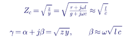
For the Keentel 345 kV model:

That is 0.074° per kilometer, or about 11.9° per 100 miles at 60 Hz. A full wavelength is about 4,870 km (3,020 miles) — close to the free-space value of 5,000 km at 60 Hz, because overhead line waves travel at about 97% of the speed of light.
2.3 Surge impedance loading

For the 345 kV model, SIL = 345² ÷ 287 ≈ 415 MW. At SIL, the line's reactive generation (charging) exactly balances its reactive consumption (I²X), and the voltage profile is flat. Below SIL, the line generates net reactive power and voltage rises toward the receiving end. The Ferranti effect is the limiting case at zero load.
3. The long-line equations
3.1 ABCD parameters
For a uniform line of length ℓ, sending-end and receiving-end quantities are related by:
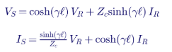
3.2 Open-circuit receiving end
With the receiving end open, IR = 0, so:
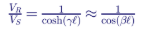
The lossless approximation is excellent for EHV lines. The voltage at any point x measured from the receiving end follows a cosine profile:
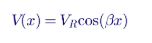
so the voltage rises continuously from the sending end to the open end, as shown in the middle panel of Figure 1.
3.3 Worked example: 217-mile, 345 kV line
| Step | Calculation | Result |
|---|---|---|
| Length | 217.5 miles | 350 km |
| Electrical length | βℓ = 1.29 × 10⁻³ × 350 | 0.452 rad = 25.9° |
| Exact (lossless) ratio | 1 ÷ cos(25.9°) | 1.1116 |
| Exact with losses (Keentel model) | 1 ÷ magnitude of cosh(γℓ) | 1.1114 |
| Receiving-end voltage for 345 kV sending | 345 × 1.111 | 383 kV |
| Maximum operating voltage of 345 kV equipment | ANSI/IEEE rated maximum | 362 kV |
The open-end voltage exceeds the 362 kV maximum operating voltage by about 6%. Energizing this line from one end without compensation is not acceptable for continuous operation.
3.4 The quick approximation
Expanding the cosine for short electrical lengths:
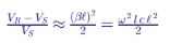
For the 217-mile line, (0.452)² ÷ 2 = 10.2%, compared with the exact 11.1%. The approximation underestimates the rise and becomes increasingly inaccurate beyond roughly 150 miles at 60 Hz. It does, however, show the two key scaling laws: the rise grows with the square of length and with the square of frequency.
3.5 Why 60 Hz matters
The same physical line has 20% more electrical length at 60 Hz than at 50 Hz. Because the rise scales roughly with the square of electrical length, it is about 45% to 50% larger at 60 Hz.
| Line length | Rise at 50 Hz | Rise at 60 Hz |
|---|---|---|
| 100 miles | 1.5% | 2.2% |
| 150 miles | 3.5% | 5.1% |
| 200 miles | 6.3% | 9.3% |
| 217 miles (350 km) | 7.5% | 11.1% |
| 250 miles | 10.1% | 15.2% |
| 300 miles | 15.2% | 23.1% |
This is the most important correction when applying international literature to US systems: 50 Hz results understate the Ferranti rise on US lines.
3.6 The quarter-wavelength limit
As βℓ approaches 90°, cos(βℓ) approaches zero and the open-end voltage tends toward infinity, limited only by losses and corona. At 60 Hz, a quarter wavelength is about 755 miles (1,215 km). No uncompensated line approaches this length in practice, but the rapid growth of the rise beyond 300 miles explains why very long EHV lines always require compensation.
3.7 Does voltage class matter?
A useful and often surprising result is that the per-unit Ferranti rise of an overhead line depends almost entirely on its length and frequency, not on its voltage class. The phase velocity of overhead lines is close to the speed of light for every voltage class, because √(lc) depends on geometry ratios that change little. What changes dramatically with voltage class is the amount of charging reactive power — and therefore the source-side rise and the size of the reactors needed.
For a 150-mile overhead line at 60 Hz:
| Voltage class | Phase shift per 100 miles (approx.) | Open-end rise, stiff source | Charging (Mvar) | Sending-end rise with 5,000 MVA source |
|---|---|---|---|---|
| 115 kV | ≈ 12° | ≈ 5% | ≈ 11 | ≈ 0.2% |
| 138 kV | ≈ 12° | ≈ 5% | ≈ 15 | ≈ 0.3% |
| 230 kV | ≈ 12° | ≈ 5% | ≈ 46 | ≈ 0.9% |
| 345 kV | ≈ 12° | ≈ 5% | ≈ 129 | ≈ 2.6% |
| 500 kV | ≈ 12° | ≈ 5% | ≈ 285 | ≈ 5.7% (source this weak is unusual at 500 kV) |
| 765 kV | ≈ 12° | ≈ 5% | ≈ 730 | Requires a much stronger source and line reactors |
The practical consequence is that Ferranti problems become severe at EHV not because the per-unit line rise is larger, but because EHV lines tend to be longer, carry far more charging, and connect to sources whose strength is small relative to that charging. At 765 kV, a single long line can draw as much charging as a large generator's entire reactive capability, which is why 765 kV lines are almost always built with line-connected reactors.
3.8 Physical intuition: the phasor picture
Consider the line as many short segments. At the open end, the last segment carries only its own small charging current. Moving toward the source, each segment carries the charging current of all segments downstream, so the current grows almost linearly toward the sending end. Each segment's inductance develops a voltage jωLI that, for a leading current, adds in phase with the local voltage. The rise accumulates from the source to the open end, and because the current is largest near the source, most of the rise happens in the first half of the line — which is exactly the shape of the uncompensated profile in Figure 1. Shunt reactors placed at the ends cancel part of the charging current where it accumulates most, which explains why end-located reactors are so effective and why the compensated profile peaks near the middle of the line.
4. The role of the source
4.1 Source impedance raises the sending end
Charging current drawn by the line flows through the source impedance, and because it is leading current, it raises the sending-end bus voltage. The rise is approximately:
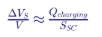
For one 345 kV, 217-mile circuit drawing about 187 Mvar of charging from a 10,000 MVA source, the sending-end rise is about 1.9%. For both circuits of a double-circuit line, charging doubles to about 375 Mvar and the sending-end rise to about 3.8%.
4.2 Combined rise relative to source voltage
The open-end voltage relative to the source's internal voltage combines both effects:
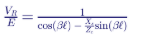
| Source short-circuit capacity | Sending-end rise | Receiving-end voltage relative to source EMF |
|---|---|---|
| Infinite (stiff) | 0% | 1.111 pu |
| 20,000 MVA | 1.0% | 1.123 pu |
| 10,000 MVA | 2.1% | 1.134 pu |
| 5,000 MVA | 4.2% | 1.158 pu |
| 2,500 MVA | 8.8% | 1.209 pu |
Energizing a long line from the weaker end produces a markedly higher open-end voltage. Operating procedures therefore normally specify energization from the stronger terminal, with the sending-end voltage reduced before closing if necessary.
4.3 Generator self-excitation
When a long line is energized from a small generator — as in black-start restoration — the line's charging can exceed the generator's underexcited reactive capability. The generator's terminal voltage can then rise uncontrollably as the line's capacitive reactance resonates with the generator's synchronous reactance. A simplified check for self-excitation risk is:

where XC,line is the capacitive reactance of the energized line seen at the generator terminals and Xd is the generator's synchronous reactance (on a common base). Restoration plans must confirm that cranking paths stay well clear of this condition, typically by energizing with shunt reactors in service, limiting the length of line energized at once and picking up load early.
5. Line modeling approaches
5.1 Nominal and equivalent pi models
The nominal pi model lumps the series impedance zℓ in a single branch and splits the shunt admittance yℓ equally between two shunt branches. It is accurate for short lines and for steady-state calculations on medium-length lines. The equivalent pi model corrects the lumped values with hyperbolic factors so that it reproduces the exact long-line solution at one frequency:

Power flow programs use equivalent pi models, so steady-state Ferranti rise calculated in a load flow is exact at 60 Hz — provided the line data are correct.
Keentel's comparison for the 217-mile line shows how cascading nominal pi sections converges:
| Number of nominal pi sections | Receiving-end ratio | Error versus exact |
|---|---|---|
| 1 | 1.1135 | +0.21 percentage points |
| 2 | 1.1119 | +0.05 |
| 5 | 1.1115 | +0.01 |
| 10 | 1.1114 | +0.003 |
| Exact distributed | 1.1114 | — |
5.2 Pi models in time-domain simulation
In EMT simulation, a cascade of pi sections represents traveling waves only approximately. Each section acts as a low-pass filter with a cutoff frequency near:
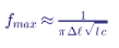
where Δℓ is the section length. A practical guideline is that each section should be shorter than about one-tenth of the shortest wavelength of interest. For switching transients with content up to several kilohertz, a 200-mile line needs many short sections, and the model still introduces spurious oscillations. Pi models are therefore best reserved for short lines or for low-frequency studies.
5.3 Bergeron (constant-parameter distributed) model
The Bergeron model represents the line as lossless traveling waves with travel time τ = ℓ√(lc) and surge impedance Zc, with resistance lumped at the ends and middle. Parameters are calculated at one frequency, usually 60 Hz. It reproduces fundamental-frequency behavior and wave travel times accurately and is computationally efficient. Its limitation is that line resistance and inductance actually change with frequency, particularly in zero sequence because of ground-return effects, so damping and wave shape at high frequencies are approximate.
The traveling-wave relationship at each terminal k of a line between nodes k and m is:

5.4 Frequency-dependent models
Frequency-dependent (FD) models fit the line's characteristic admittance and propagation function over a wide frequency range, either in modal form or directly in the phase domain (the universal line model used in modern EMT programs). They capture:
- the strong frequency dependence of zero-sequence resistance and inductance due to earth return,
- skin effect in conductors and ground wires,
- untransposed geometry and mutual coupling between circuits on the same towers,
- realistic damping of switching transients.
FD models are the preferred choice for switching overvoltage studies, transient recovery voltage, secondary arc and single-pole tripping studies, and resonance studies involving double-circuit coupling.
5.5 Model selection summary
| Study | Pi (nominal or equivalent) | Bergeron | Frequency-dependent |
|---|---|---|---|
| Steady-state Ferranti rise | Adequate (equivalent pi exact at 60 Hz) | Adequate | Adequate |
| Load flow and voltage control | Standard | Not used | Not used |
| Energization and reclosing overvoltages | Not recommended for long lines | Acceptable for screening | Preferred |
| Transient recovery voltage | Not recommended | Acceptable with care | Preferred |
| Secondary arc and single-pole reclosing | Not recommended | Limited | Preferred |
| Harmonic and resonance studies | Equivalent pi at each frequency, or FD | Limited | Preferred |
| Untransposed and double-circuit coupling | Possible with coupled sections | Possible | Preferred |
The published 50 Hz comparison reviewed in Part A illustrates the first row: all models agreed within 0.13 percentage points on steady-state rise. That agreement should not be extrapolated to transient studies, where the models can differ substantially in peak overvoltage and damping.
6. From steady-state rise to switching overvoltage
6.1 Energization transients
When a breaker closes onto an open line, a voltage step travels down the line at nearly the speed of light, reflects at the open end and doubles. The reflected wave returns to the source, reflects again and continues to bounce, superimposed on the rising steady-state voltage. The peak transient voltage at the open end depends on:
| Factor | Effect on peak overvoltage |
|---|---|
| Point on wave at closing | Closing at voltage peak produces the largest step |
| Trapped charge (high speed reclosing) | Can raise peaks toward 3 pu or more |
| Steady-state Ferranti rise | Raises the base on which transients ride |
| Source strength and network | Determines wave reflections at the sending end |
| Breaker pole scatter | Causes coupled transients between phases |
| Line losses and frequency dependence | Damp transients |
| Mitigation (pre-insertion resistors, controlled switching, arresters) | Can limit peaks to about 1.5 to 2.0 pu |
In Keentel's single-phase-equivalent EMT model of the 217-mile line, closing at a voltage peak from a 10,000 MVA source produces a peak of about 2.2 pu at the open end. Closing at a voltage zero limits the peak to about 1.6 pu. Three-phase studies with realistic breaker pole scatter and statistical switching typically show 2% switching overvoltages of 2.0 to 2.8 pu for unmitigated EHV line energization, and higher for reclosing onto trapped charge.
6.2 Insulation coordination
IEEE 1313.1 and IEEE 1313.2 define the insulation coordination process. For EHV lines, switching surge performance often controls tower clearances and insulator string length. The steady-state Ferranti rise, the temporary overvoltages it creates and the switching surge distribution must be considered together:
| Voltage class | Maximum operating voltage | Typical controlled switching overvoltage target |
|---|---|---|
| 345 kV | 362 kV | About 2.0 to 2.2 pu |
| 500 kV | 550 kV | About 1.8 to 2.0 pu |
| 765 kV | 800 kV | About 1.6 to 1.8 pu |
7.2 Detuning ratios for 60 Hz systems
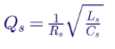

7.2 Detuning ratios for 60 Hz systems
| Reactor ratio p | Tuning order | Tuning frequency at 60 Hz | Tuning frequency at 50 Hz (reference only) | Typical use |
|---|---|---|---|---|
| 5.67% | 4.20 | 252 Hz | 210 Hz | Common in US practice for 5th-dominant systems; branch absorbs some 5th current |
| 7% | 3.78 | 227 Hz | 189 Hz | Conservative detuning for 5th and higher; less absorption |
| 14% | 2.67 | 160 Hz | 134 Hz | Systems with significant 3rd harmonic (single-phase loads, unbalanced loads) |
Using 50 Hz tuning frequencies in a US design is a common and costly error. A designer who looks up "7% equals 189 Hz" and compares it with 300 Hz for the 5th harmonic gets the right conclusion for the wrong reason; one who applies a 50 Hz table to select a ratio for a target frequency gets the wrong reactor.
7.3 Capacitor voltage rise
The series reactor raises the fundamental voltage across the capacitor:
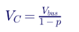
For a 480 V bus with 7% detuning, VC = 480 ÷ 0.93 = 516 V. Harmonic voltages add to this. Capacitors in detuned banks must therefore be rated above system voltage — typically 525 V or 600 V units on a 480 V system, and correspondingly higher ratings at medium voltage.
7.4 Effective kvar output
The output of a detuned step depends on the capacitor's rated voltage and the detuning ratio:

A 600 kvar, 525 V capacitor step with 7% detuning on a 480 V bus delivers about 600 × (480 ÷ 525)² ÷ 0.93 ≈ 539 kvar. Designers who specify detuned banks by nameplate capacitor kvar without this correction will under- or over-compensate.
7.5 The resonance that detuning creates
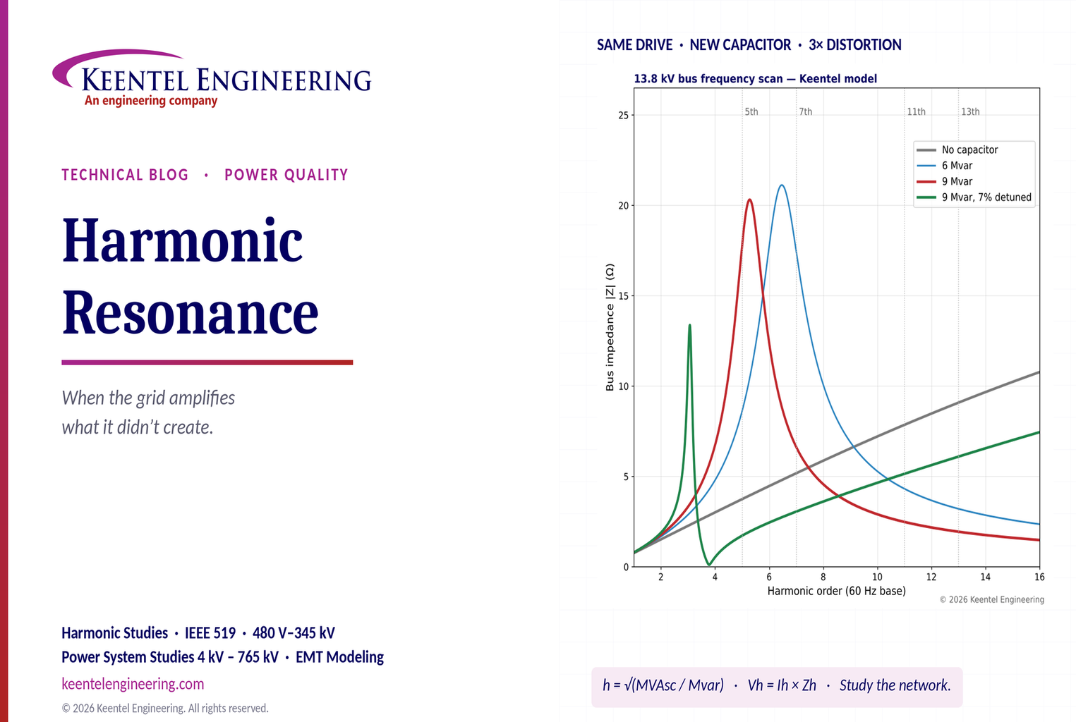
A detuned bank does not eliminate parallel resonance. It moves the combined network resonance below the branch tuning frequency. In Keentel's 13.8 kV model, the 7% detuned 9 Mvar bank produces a parallel resonance near the 3.1st harmonic. That is harmless if 3rd harmonic current is negligible — usually true on a balanced three-wire 13.8 kV bus with six-pulse drives. It can be harmful at 480 V or 208 V buses with large single-phase loads or unbalance, where 3rd harmonic current flows. In those cases a 14% ratio, tuning at 160 Hz, keeps the resonance below the 3rd.
7.6 What detuned reactors are not
Detuned reactors protect the capacitor bank and prevent it from creating a resonance at characteristic harmonics. They are not harmonic filters. A 7% detuned bank absorbs only a modest share of 5th harmonic current. If a facility must reduce harmonic current to meet IEEE 519 at the point of common coupling, a tuned filter or active harmonic filter is usually needed.
8. Tuned passive filters
8.1 Single-tuned filters
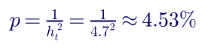
A single-tuned filter deliberately creates a low-impedance series path at a specific harmonic, slightly below it to allow for capacitor tolerance, temperature drift and aging. For the 5th harmonic, tuning near 4.7th is typical. The reactor ratio is:
8.2 Worked example: 9 Mvar, 13.8 kV 5th harmonic filter
| Quantity | Calculation | Result |
|---|---|---|
| Capacitor reactance | 13.8² ÷ 9 | 21.16 Ω |
| Reactor reactance at 60 Hz | 21.16 × 4.7% | 0.958 Ω |
| Reactor inductance | 0.958 ÷ (2π × 60) | 2.54 mH |
| Capacitor fundamental voltage | 13.8 ÷ (1 − 0.0453) | 14.45 kV line-to-line (rate capacitors accordingly) |
| Quality factor (typical) | XL at tuning ÷ R | 30 to 60 |
The filter still forms a parallel resonance with the source, now below 4.7th. The design must confirm that this resonance does not coincide with any harmonic present, including non-characteristic harmonics from unbalance and transformer inrush.
8.3 Filter duty and absorption
A tuned filter absorbs harmonic current not only from the plant's drives but from the entire utility system. A filter designed only for the plant's own harmonic load can be overloaded by background distortion. IEEE 1531 describes the design process, including background distortion, detuning, unbalance protection and ratings of each component.
8.4 Damped and high-pass filters
Second-order high-pass and C-type filters provide damping across a band rather than a single sharp notch. They are common at transmission and collector levels, where the resonant frequency may move with network configuration and a sharp notch could create new resonances. C-type filters avoid fundamental-frequency losses in the damping resistor by tuning an auxiliary branch to fundamental frequency.
9. Active harmonic filters and network impedance
Active harmonic filters (AHFs) inject harmonic currents in opposition to load harmonics, measured through current transformers. They are effective for variable loads and for multiple harmonic orders. However, they are not a substitute for understanding network impedance:
| Issue | Why it matters |
|---|---|
| Limited control bandwidth | AHFs compensate up to a maximum harmonic order, typically the 50th; resonances above that range are unaffected |
| Rating limits | At resonance, harmonic currents may exceed AHF capacity, causing the AHF to saturate and stop compensating effectively |
| CT location | Compensating load current does not address distortion imported from the supply or circulating between capacitors and the source |
| Interaction with capacitors | Capacitors downstream of AHF current measurement can create resonances the AHF cannot see or may amplify |
| Control stability | AHF controls interact with network impedance; in some cases they can excite resonances near their switching or control bandwidth |
| Switching-frequency emissions | AHFs and active front ends emit at 2 kHz to 20 kHz; cable capacitance and capacitors can resonate there |
An AHF should be specified after a frequency scan of the network, with its rating, CT location and control settings selected for the actual resonance conditions.
10. Equipment duty
10.1 Capacitor limits under IEEE 18
IEEE Std 18 specifies continuous operating limits for shunt power capacitors, including harmonic content:
| Quantity | IEEE 18 continuous limit |
|---|---|
| RMS voltage | 110% of rated |
| Crest (peak) voltage | 120% of rated √2 voltage |
| RMS current | 135% of nominal current at rated voltage and frequency |
| Reactive power | 135% of rated kvar |
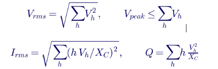
Duty quantities are calculated by summing harmonic components:
10.2 Worked example: duty of the 9 Mvar bank in resonance
Using the harmonic voltages from Keentel's scan for the 9 Mvar case at nominal fundamental voltage:
| Quantity | Calculated value | IEEE 18 limit | Assessment |
|---|---|---|---|
| RMS voltage | 1.003 pu | 1.10 pu | Within limit |
| Peak voltage (arithmetic sum, worst case) | 1.10 pu | 1.20 pu | Within limit, small margin if fundamental voltage is high |
| RMS current | 1.075 pu | 1.35 pu | Within limit |
| Reactive power | 1.03 pu | 1.35 pu | Within limit |
This result is instructive. The capacitor bank itself is within its IEEE 18 ratings, yet the bus voltage THD of 7.7% exceeds the IEEE 519 limit of 5% for 13.8 kV buses. Equipment damage is not the only consequence of resonance; voltage quality for every load on the bus is. With operating voltage at 105% and a lighter load (less damping), the margins on peak voltage and current shrink rapidly. Capacitor fuses — sized with modest margin over fundamental current — and capacitor units with manufacturing tolerances or aging can fail long before the bank as a whole reaches its limits.
10.3 Transformers
Harmonic currents increase transformer eddy-current and stray losses, which rise roughly with the square of harmonic order. IEEE C57.110 provides the harmonic loss factor method for derating:
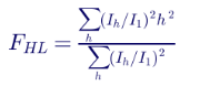
A transformer carrying amplified 5th and 7th harmonic currents in series resonance can overheat at a fundamental load well below nameplate.
10.4 Drives, UPS and electronic loads
Voltage distortion flattens or peaks the voltage waveform. Six-pulse drives charge their DC link from the voltage peaks; a peaked waveform raises DC bus voltage and can cause overvoltage trips, while a flattened waveform reduces it and can cause undervoltage trips under load. Distortion can also disturb zero-crossing detection in thyristor controls, synchronization of UPS and generator systems, and the operation of sensitive instrumentation.
10.5 Cables, motors and metering
Harmonic currents increase cable heating through skin and proximity effects. Negative-sequence harmonics (5th, 11th) create counter-rotating torque in motors, raising losses and vibration. Revenue meters and protective relays may respond differently to distorted waveforms, causing billing disputes or protection misoperation.
11. IEEE 519-2022 limits
IEEE 519-2022 sets harmonic limits at the point of common coupling (PCC) — the point where the utility serves multiple customers, or as agreed between the user and utility.
11.1 Voltage distortion limits
| Bus voltage at PCC | Individual harmonic | Voltage THD |
|---|---|---|
| 1 kV and below | 5.0% | 8.0% |
| Above 1 kV through 69 kV | 3.0% | 5.0% |
| Above 69 kV through 161 kV | 1.5% | 2.5% |
| Above 161 kV | 1.0% | 1.5% |
In US voltage classes: 480 V and 600 V buses fall in the first row; 4.16 kV, 13.8 kV, 34.5 kV and 69 kV in the second; 115 kV and 138 kV in the third; 230 kV, 345 kV, 500 kV and 765 kV in the fourth.
11.2 Current distortion limits (120 V through 69 kV)
| Isc/IL | h < 11 | 11 ≤ h < 17 | 17 ≤ h < 23 | 23 ≤ h < 35 | 35 ≤ h ≤ 50 | TDD |
|---|---|---|---|---|---|---|
| < 20 | 4.0% | 2.0% | 1.5% | 0.6% | 0.3% | 5.0% |
| 20 to < 50 | 7.0% | 3.5% | 2.5% | 1.0% | 0.5% | 8.0% |
| 50 to < 100 | 10.0% | 4.5% | 4.0% | 1.5% | 0.7% | 12.0% |
| 100 to < 1000 | 12.0% | 5.5% | 5.0% | 2.0% | 1.0% | 15.0% |
| > 1000 | 15.0% | 7.0% | 6.0% | 2.5% | 1.4% | 20.0% |
Even harmonics are limited to 25% of the odd harmonic limits. The 2022 edition also allows defined percentages of time above the limits (for example, statistical evaluation using very-short-time and short-time values) and provides adjustments for low-order harmonics in certain conditions. The current limits apply to the user's emissions; the voltage limits are the shared responsibility of user and utility.
11.3 Why resonance complicates compliance
IEEE 519 compliance is assessed at the PCC, but resonance inside a facility can cause problems that never violate PCC limits, and a utility-side resonance can cause PCC voltage limits to be exceeded even when every customer meets its current limits. Compliance and reliability are related but not the same question.
12. Credible operating configurations
Resonance studies must consider every credible configuration, not just the design case.
| Configuration change | Effect on resonance |
|---|---|
| Capacitor stages switched in or out | More capacitance lowers the resonance; automatic controllers sweep it through a range |
| Transformers paralleled or tie breakers closed | Lower source inductance raises the resonance; may move it from 5th to 7th |
| Transformers with different impedances in parallel | Changes both the resonance and the current sharing at harmonic frequencies |
| Utility source changes (alternate feed, upstream outage, generation changes) | Changes short-circuit capacity and moves the resonance |
| On-site generators running | Generator subtransient reactance changes source impedance |
| New MV cable runs | Adds distributed capacitance; long cables may create resonances on their own |
| Load level changes (night, weekend, process shutdown) | Reduces damping; peaks rise |
| New converter loads or retrofits | Adds harmonic sources; may remove resistive damping |
| Utility capacitor bank switching nearby | Changes background impedance and distortion |
13. A practical investigation and study workflow
- Collect data: one-line diagrams, transformer nameplates, cable lengths and types, capacitor banks and controls, drive and converter inventory, utility short-circuit data (maximum and minimum) and utility capacitor banks near the PCC.
- Measure: install power quality monitors at the PCC, main buses and suspected equipment, recording harmonic voltages and currents with phase angles over at least a week of representative operation. Use measurement methods consistent with IEEE 1159 and IEEE 519-2022.
- Build the harmonic model: frequency-dependent models of sources, transformers, cables, capacitors, motors, loads and harmonic sources in a harmonic analysis program.
- Run frequency scans: driving-point impedance at key buses and transfer impedances between buses for every credible configuration.
- Run harmonic load flows: calculate harmonic voltages and currents for each configuration with realistic harmonic spectra.
- Validate the model: compare calculated distortion with measurements for the configurations observed in the field. Adjust source impedance, load damping and harmonic spectra as needed.
- Check equipment duty: capacitors (IEEE 18), filters (IEEE 1531), transformers (IEEE C57.110), cables, drives and protective devices.
- Design mitigation: detuned or tuned banks, filters, AHFs, configuration limits or source changes.
- Verify after installation: measure again and confirm that distortion and duty match predictions.
13.1 Digital twins and EMT simulation
For complex systems — large data centers, inverter-based plants, facilities with many converters — frequency-domain models can be supplemented by electromagnetic transient (EMT) simulations. EMT models capture capacitor switching transients, transformer inrush, converter control behavior and nonlinear interactions that frequency-domain methods simplify. A validated model, kept current as the facility changes, becomes a digital twin that can screen future additions before they are installed.
14. Resonance in inverter-based plants and data centers
14.1 Solar, wind and storage collector systems
Utility-scale plants use long 34.5 kV collector cables, inverter step-up transformers, a main power transformer to 115 kV, 138 kV, 230 kV or 345 kV, and sometimes shunt capacitor banks or harmonic filters. Cable capacitance resonating with transformer inductance typically produces resonances in the range of several hundred hertz to a few kilohertz. Background harmonic distortion from the transmission system can be amplified into the plant, and inverter emissions can be amplified out to the POI. Transmission providers increasingly require harmonic studies demonstrating IEEE 519 compliance at the POI.
14.2 Data centers
Data centers combine large UPS and server power supply loads, MV cable networks within the campus, power factor correction (sometimes integrated in UPS systems), on-site generators, and increasingly BESS and on-site generation. Modern UPS and power supplies with active front ends produce low low-order harmonics but emit near their switching frequencies. Generator operation raises source impedance dramatically compared with utility supply, moving resonances lower and increasing distortion during generator operation — a configuration that must be studied separately.
14.3 EV charging hubs
DC fast chargers aggregate tens of megawatts of converter load at a single service. Charger designs vary, and the combination of chargers from different vendors, service transformers and any site capacitors or storage converters creates resonances that must be studied as the hub grows.
14A. Capacitor switching, inrush and resonance
Resonance is a steady-state frequency-domain concept, but the same inductance and capacitance also govern switching transients. When a capacitor bank is energized, the network rings at its natural frequency — which is the same parallel resonant frequency identified in a frequency scan. Two effects deserve attention.
Magnification of switching transients
When a utility switches a large capacitor bank on its system, an oscillatory transient at a few hundred hertz propagates down the feeder. If a customer's low-voltage capacitor bank and service transformer form a series circuit tuned near that transient frequency, the transient voltage at the customer bus can be magnified to two to four times its normal peak. Drives with diode front ends are especially vulnerable: the DC link capacitor charges through the surge and trips the drive on DC overvoltage. The classic remedy is to add input reactance (line reactors or DC chokes) to drives, convert the customer bank to a detuned bank, or ask the utility to use synchronous closing or pre-insertion devices on its bank.
Back-to-back switching inrush
When one capacitor stage is energized next to stages already in service, the inrush current is limited only by the small inductance between them. The peak inrush current and frequency for back-to-back switching are approximately:

where Ceq is the series combination of the switched and energized capacitances and Leq is the inductance between them. Inrush frequencies of several kilohertz and peaks of many times rated current are common. IEEE C37.012 and IEEE 1036 provide guidance on limiting reactors and switching device capability. A detuned reactor in each step also limits back-to-back inrush — a secondary benefit that is often overlooked.
Transformer energization and the 2nd harmonic
Transformer inrush current is rich in the 2nd harmonic and also contains odd harmonics. If a network has a parallel resonance near the 2nd or 3rd harmonic — as happens with heavily detuned banks or very large capacitance relative to source strength — energizing a transformer can excite sustained resonant overvoltage that decays slowly. This temporary overvoltage can stress surge arresters and delay relay restraint. EMT studies are the appropriate tool when a resonance below the 4th harmonic is identified at a bus where large transformers are energized.
14B. Worked example: should the plant buy an active filter or a detuned bank?
A 480 V plant has 900 kW of six-pulse drive load and a 2,000 kVA, 5.75% transformer. It wants both power factor correction (about 600 kvar) and compliance with an IEEE 519 TDD limit of 8% at its 13.8 kV PCC, where ISC/IL is about 35.
| Option | Harmonic result | Resonance risk | Approximate considerations |
|---|---|---|---|
| Plain 600 kvar automatic bank | Current TDD unchanged or worse; resonance near the 7.6th with all steps in | High: steps sweep the resonance across the 7th | Lowest cost, highest risk |
| 600 kvar bank, 7% detuned | TDD reduced modestly by partial 5th absorption | Low at characteristic harmonics; new resonance near the 3rd | Moderate cost; PF goal met; may not meet TDD alone |
| Active harmonic filter sized for drive harmonics, plus 7% detuned bank | TDD reduced below the limit | Low, provided the AHF CTs are located upstream of the detuned bank and the AHF is not asked to compensate bank currents | Higher cost; meets both goals |
| Drives replaced or retrofitted with active front ends | TDD very low at low orders | Check emissions near switching frequency | Highest cost; long-term best where drives are due for replacement |
The engineering point is that the decision depends on the resonance analysis. A plain bank — the cheapest line in the table — is the one most likely to create the problem the plant is trying to avoid. Keentel's practice is to select the option by modeling all four alternatives in every credible configuration, then confirming the chosen option with measurements after installation.
15. Common misconceptions corrected
| Misconception | Engineering reality |
|---|---|
| "Harmonics come from the equipment, so fix the equipment." | The network determines how harmonic currents become harmonic voltages and where currents flow. Fixing the source without studying the network can leave the resonance in place. |
| "Capacitors absorb harmonics, so they help." | Unfiltered capacitors often create resonances that amplify harmonics. Only tuned branches absorb harmonics in a controlled way. |
| "Detuned reactors are harmonic filters." | Detuned reactors protect the capacitor and avoid resonance at characteristic harmonics; they absorb relatively little harmonic current. |
| "An active filter makes a network study unnecessary." | AHF rating, bandwidth and CT location must suit the actual network impedance and resonances. |
| "If we met IEEE 519 at commissioning, we are done." | Configuration changes, new loads, utility changes and capacitor switching can create new resonances later. |
| "The 50 Hz detuning table applies everywhere." | US systems are 60 Hz; tuning frequencies are 20% higher for the same ratio. |
| "A meter showing high harmonic current at a facility proves the facility is the source." | Series resonance can make a facility draw large harmonic currents from upstream distortion. Phase angle analysis is needed. |
| "Resonance is a fault." | Resonance is a network property. It becomes a problem only when it coincides with harmonic sources and insufficient damping. |
16. Key takeaways
- The network matters as much as the harmonic source. Vh = Ih × Zh, and Zh is set by the network.
- Parallel resonance amplifies voltage; series resonance amplifies current. Both can occur in the same facility.
- Estimate first, then scan. hr = √(MVAsc ÷ Mvar) gives a fast warning; frequency scans and harmonic load flows confirm.
- Study every credible configuration. Capacitor stages, transformer paralleling, source changes and load levels all move the resonance.
- Use 60 Hz numbers. ft = 60 ÷ √p for detuned and tuned banks in the US.
- Check equipment duty and voltage quality. IEEE 18, IEEE 1531, IEEE C57.110 and IEEE 519-2022 each address a different part of the problem.
- Verify in the field. Measurement before and after mitigation closes the loop.
17. How Keentel Engineering helps
Keentel Engineering performs power quality and harmonic studies for industrial plants, data centers, water and wastewater utilities, EV charging hubs, solar, wind and storage plants and electric utilities, from 480 V to 765 kV.
| Stage | Keentel scope | Outcome |
|---|---|---|
| Power quality investigation | Measurement planning, monitor installation, data analysis and root cause | Clear diagnosis of the source and the network's role |
| Harmonic modeling | Frequency-dependent models of sources, transformers, cables, capacitors and loads | Accurate, validated harmonic model |
| Frequency scans and harmonic load flow | All credible configurations, including capacitor stages, transformer ties and generator operation | Identification of resonances before they cause damage |
| Equipment duty assessment | Capacitors (IEEE 18), filters (IEEE 1531), transformers (IEEE C57.110), cables and drives | Confirmation that equipment is properly rated |
| Mitigation design | Detuned banks, tuned and damped filters, AHF specification, configuration limits | Cost-effective solutions that suit the network |
| IEEE 519 compliance | PCC assessment and documentation for utilities and transmission providers | Compliance with supporting evidence |
| Inverter-based plant harmonics | Collector system and POI harmonic studies, EMT studies | Interconnection approval and reliable operation |
| Verification | Post-installation measurement and model updates | Proof that mitigation works |
Why clients choose Keentel Engineering
- System-level thinking: we study the network, not only the equipment.
- From measurement to design: field data, models and engineered solutions under one team.
- Utility and industrial experience: practical knowledge of utility requirements and facility operations.
- Inverter-based resource expertise: harmonic and EMT studies for solar, wind and storage interconnections.
- Licensed professional engineering: a Florida-registered firm with offices in Tampa, Austin, Sacramento and Baltimore, supporting projects nationwide.
Capacitor fuses operating, transformers running hot or drives tripping without explanation? Talk to Keentel Engineering at (813) 389-7871, contact@keentelengineering.com, or book a 15-minute scoping call at calendly.com/keentel-engineering/15min.
Part C — Case Studies
The following are illustrative scenarios based on conditions typical of US facilities and interconnections. They show how Keentel Engineering approaches harmonic resonance problems; site details are generalized and figures are rounded.
Case Study 1 — 480 V food processing plant: capacitor fuses and drive trips
Situation. A food processing plant supplied by a 2,000 kVA, 13.8 kV to 480 V transformer installs a 1,200 kvar automatic power factor correction bank in four 300 kvar steps. Within weeks, capacitor fuses operate repeatedly, the transformer runs hot, and several conveyor and pump drives trip on DC bus overvoltage, usually during evening shifts when process heating is off.
Analysis. Keentel installs power quality monitors on the main bus and the capacitor bank. With all four steps in service, 5th harmonic voltage reaches 9% and capacitor current reaches 140% of rated during light-load periods. Hand calculation and a frequency scan show the parallel resonance moving from the 10.8th harmonic with one step to about the 5.4th with four steps — and closer still when the utility source impedance is included. Evening loss of resistive heating load reduces damping and sharpens the peak.
Engineered solution. Keentel specifies replacement of the bank with a 7% detuned automatic bank using 525 V capacitors, sized for an effective 1,100 kvar after accounting for voltage rise and detuning. The design confirms that the new network resonance near the 3rd harmonic does not coincide with significant 3rd harmonic current, which measurements show to be small on the three-wire 480 V system.
Outcome. Voltage THD falls below 4%, capacitor fuse operations stop, drive trips cease, and the plant retains its power factor improvement.
Case Study 2 — 13.8 kV water treatment plant: the second transformer
Situation. A water treatment plant has two 13.8 kV buses, each fed by a 115 kV to 13.8 kV transformer, with a normally open tie breaker. Large pump drives and a 6 Mvar capacitor bank are on Bus A. During a planned maintenance outage, operators close the tie and run both buses from one transformer, then later parallel both transformers. Pump drives on Bus B begin tripping, and power quality alarms report high 7th harmonic distortion.
Analysis. Keentel builds a harmonic model for every credible configuration: buses split, tie closed with one transformer, and tie closed with both transformers paralleled. With buses split, Bus A resonance is near the 6.5th harmonic — high distortion but within limits because of load damping. Paralleling the transformers lowers source impedance and moves the resonance to about the 7.4th, while the tie adds Bus B's drives as additional 7th harmonic sources. Measured 7th harmonic voltage exceeds 5%.
Engineered solution. Keentel recommends converting the 6 Mvar bank to a 5th harmonic tuned filter at the 4.7th harmonic, with a reactor and capacitors rated for background distortion and both configurations, and develops an operating procedure for tie operation until the filter is installed.
Outcome. Distortion remains below IEEE 519 limits in all configurations, the plant can use its tie breaker flexibly, and maintenance outages no longer cause drive trips.
Case Study 3 — 200 MW solar plant at 138 kV: amplified background distortion
Situation. A 200 MW solar plant with a 34.5 kV collector system connects to a 138 kV substation. After the utility installs a new 138 kV capacitor bank at a nearby substation, the plant's POI meter shows 13th harmonic voltage above the IEEE 519 individual limit of 1.5% for that voltage class, and the transmission provider asks the plant to investigate.
Analysis. Keentel's measurements show 13th harmonic current flowing into the plant from the 138 kV system, not out of it. A frequency scan of the plant and surrounding network reveals a parallel resonance near the 13th harmonic formed by the collector cable capacitance, the main power transformer and the new utility capacitor bank's effect on the system impedance. The plant's inverters are minor 13th harmonic sources; the resonance is amplifying existing background distortion.
Engineered solution. Keentel presents the analysis to the transmission provider with measured harmonic power flow direction and the frequency scan. The solution combines a damped high-pass filter at the plant's 34.5 kV bus, sized for background distortion, and an adjustment to the inverters' harmonic damping settings recommended by the inverter vendor.
Outcome. 13th harmonic voltage at the POI falls below 1%, the transmission provider accepts the study, and the plant avoids curtailment while the utility updates its own capacitor bank switching practice.
Part D — Technical FAQ: Harmonic Resonance
A condition where the network's inductance and capacitance produce either very high impedance (parallel resonance) or very low impedance (series resonance) at a harmonic frequency, amplifying harmonic voltage or current.
Parallel resonance raises the impedance seen by a harmonic current source and amplifies harmonic voltage. Series resonance lowers the impedance of a specific path and amplifies harmonic current driven by an existing harmonic voltage.
Use hr = √(MVAsc ÷ Mvar) at the capacitor bus, or hr ≈ √(kVA ÷ (kvar × Z)) for a low-voltage bus fed by a transformer from a strong source. Multiply by 60 Hz to get the frequency.
The 5th is usually the largest harmonic from six-pulse drives and rectifiers. A resonance near it multiplies the most significant harmonic current into a large voltage or current.
A measure of how sharp and high the resonance peak is. For a parallel resonance Q = R√(C/L); the impedance at resonance is about Q times the reactance of each element. Higher damping gives lower Q.
Resistive loads provide damping. When they are off — at night, weekends or during shutdowns — Q rises and the resonance peak becomes larger.
Yes. A transformer and capacitor bank can form a series resonance that draws amplified harmonic current from distortion already on the utility system.
A capacitor bank with a series reactor in each step, tuned below the lowest significant harmonic so the step is inductive at characteristic harmonics and cannot resonate with the source at those frequencies.
f = 60 ÷ √0.07 ≈ 227 Hz, or the 3.78th harmonic. The often-quoted 189 Hz applies only to 50 Hz systems.
The series reactor raises the fundamental capacitor voltage by 1 ÷ (1 − p). With 7% detuning at 480 V, the capacitor sees about 516 V before harmonics are added.
No. It creates a network resonance below its tuning frequency. That resonance must not coincide with harmonics present, such as the 3rd harmonic in systems with single-phase loads.
When significant 3rd harmonic current is present, for example on 208 V or 480 V systems with large single-phase loads or unbalance. A 14% ratio tunes to 160 Hz, below the 180 Hz 3rd harmonic.
A detuned bank is tuned well below the harmonics to avoid resonance and absorbs little harmonic current. A tuned filter is tuned close to a harmonic, typically the 4.7th for the 5th, to absorb that harmonic.
Their low impedance at the tuned frequency attracts harmonic current from every source connected to the network, including the utility. Filters must be rated for background distortion.
An AHF can reduce harmonic currents from loads it measures, but its rating, control bandwidth and CT location limit its effectiveness. It should be specified after a network frequency scan.
For buses above 1 kV through 69 kV, individual harmonics must be no more than 3% and voltage THD no more than 5%, evaluated statistically at the point of common coupling.
110% rms voltage, 120% peak voltage, 135% rms current and 135% reactive power, including harmonic components.
They reduce source impedance and raise the resonant frequency, which can move resonance from one harmonic to another — for example from near the 5th to near the 7th.
Power quality monitors for measurement, harmonic analysis programs for frequency scans and harmonic load flows, and EMT simulation for switching transients and converter interactions.
Focusing only on the harmonic source and the design configuration, without frequency scans of every credible configuration and field verification.
References and Further Reading
Links were current at publication (October 2026).
- IEEE Std 519-2022, Standard for Harmonic Control in Electric Power Systems. IEEE.
- IEEE Std 18-2012, Standard for Shunt Power Capacitors. IEEE.
- IEEE Std 1531-2020, Guide for the Application and Specification of Harmonic Filters. IEEE.
- IEEE Std 1036-2020, Guide for the Application of Shunt Power Capacitors. IEEE.
- IEEE Std C57.110-2018, Recommended Practice for Establishing Liquid-Immersed and Dry-Type Power and Distribution Transformer Capability When Supplying Nonsinusoidal Load Currents. IEEE.
- IEEE Std 1159-2019, Recommended Practice for Monitoring Electric Power Quality. IEEE.
- IEEE Std 399, Recommended Practice for Industrial and Commercial Power Systems Analysis (Brown Book), harmonic analysis chapter. IEEE.
- R. C. Dugan, M. F. McGranaghan, S. Santoso and H. W. Beaty, Electrical Power Systems Quality, McGraw-Hill.
- J. Arrillaga and N. R. Watson, Power System Harmonics, Wiley.
Disclaimer
This article is general technical information for educational purposes. It is not engineering advice for any specific project and does not create a professional relationship. The frequency scan results come from Keentel Engineering's simplified illustrative model; actual resonances and distortion depend on site-specific source impedance, equipment, loads and operating configurations and must be verified by project-specific study and measurement. Designs must follow current IEEE standards, the NEC, utility and transmission provider requirements and project-specific engineering analysis, sealed by a licensed professional engineer where required.
Case studies are illustrative scenarios based on typical project conditions, not records of specific client projects. Figures are rounded and indicative.
IEEE and other names are the property of their respective owners. Keentel Engineering is not affiliated with or endorsed by these organizations or any equipment vendor.
| Office | Address | Phone |
|---|---|---|
| Head Office — Tampa | 400 N Ashley Dr STE #2600, Tampa FL 33602 | (813) 389-7871 |
| Austin | 5900 Balcones Drive STE 100, Austin TX 78731 | (512) 591-0752 |
| Sacramento | 1401 21st St Ste R, Sacramento CA 95811 | (916) 913-4524 |
| Baltimore | 306 W Redwood St STE 200, Baltimore MD 21201 | (410) 225-2181 |

About the Author:
Sandip "Sonny" R. Patel, P.E.
IEEE Senior Member · Founder & CEO, Keentel Engineering
In 1995, Sonny Patel earned his Electrical Engineering degree from the University of Illinois. But degrees don't build legacies — action does.
For three decades, he has worked the power industry from every side of the table: 16 years as a utility engineer at Exelon/Commonwealth Edison; generation leadership across hydroelectric, industrial steam turbine, and a 9 GW renewable fleet; NERC Regional Entity Senior Compliance Engineer and Audit Team Lead, auditing some of the nation's largest utilities; and testing and commissioning lead on equipment up to 765 kV — the very top of the North American grid.Utility. Generator. Regulator. Consultant. Few engineers have seen all four seats. Fewer still have sat in them.
His experience spans nuclear, hydro, conventional generation, renewables, oil and gas, mining — and today's data centers, where he is authoring a three-book series on data center design. He is a Licensed Professional Engineer in six states and a Licensed Electrical Contractor in Florida (Unlimited EC) — he doesn't just design the work; he's qualified to stand behind its execution.Today, as Founder and CEO of Keentel Engineering, Sonny leads a nationwide team of engineers delivering substation design, power system studies, NERC compliance, and commissioning — done right, coast to coast.Three decades. Every side of the table. One standard: accountable engineering.
Services

Let's Discuss Your Project
Let's book a call to discuss your electrical engineering project that we can help you with.
About the Author:
Sandip "Sonny" R. Patel, P.E.
IEEE Senior Member · Founder & CEO, Keentel Engineering
In 1995, Sonny Patel earned his Electrical Engineering degree from the University of Illinois. But degrees don't build legacies — action does.
For three decades, he has worked the power industry from every side of the table: 16 years as a utility engineer at Exelon/Commonwealth Edison; generation leadership across hydroelectric, industrial steam turbine, and a 9 GW renewable fleet; NERC Regional Entity Senior Compliance Engineer and Audit Team Lead, auditing some of the nation's largest utilities; and testing and commissioning lead on equipment up to 765 kV — the very top of the North American grid.
Utility. Generator. Regulator. Consultant. Few engineers have seen all four seats. Fewer still have sat in them.
His experience spans nuclear, hydro, conventional generation, renewables, oil and gas, mining — and today's data centers, where he is authoring a three-book series on data center design. He is a Licensed Professional Engineer in six states and a Licensed Electrical Contractor in Florida (Unlimited EC) — he doesn't just design the work; he's qualified to stand behind its execution.
Today, as Founder and CEO of Keentel Engineering, Sonny leads a nationwide team of engineers delivering substation design, power system studies, NERC compliance, and commissioning — done right, coast to coast.Three decades. Every side of the table. One standard: accountable engineering.
Leave a Comment
Thank you for contacting us.
We will get back to you as soon as possible.
We will get back to you as soon as possible.
Oops, there was an error sending your message.
Please try again later.
Please try again later.
Related Posts
By SANDIP R PATEL
•
October 21, 2026
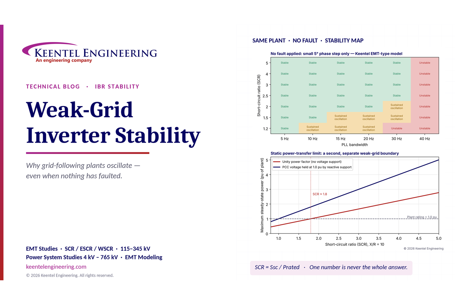
Learn why grid-following inverters become unstable without grid faults. Explore SCR, PLL interactions, EMT studies, grid strength, and mitigation.
By SANDIP R PATEL
•
October 21, 2026
Learn how harmonic resonance amplifies distortion in power systems. Explore capacitor banks, detuned reactors, frequency scans, and IEEE 519 solutions.
By SANDIP R PATEL
•
October 20, 2026
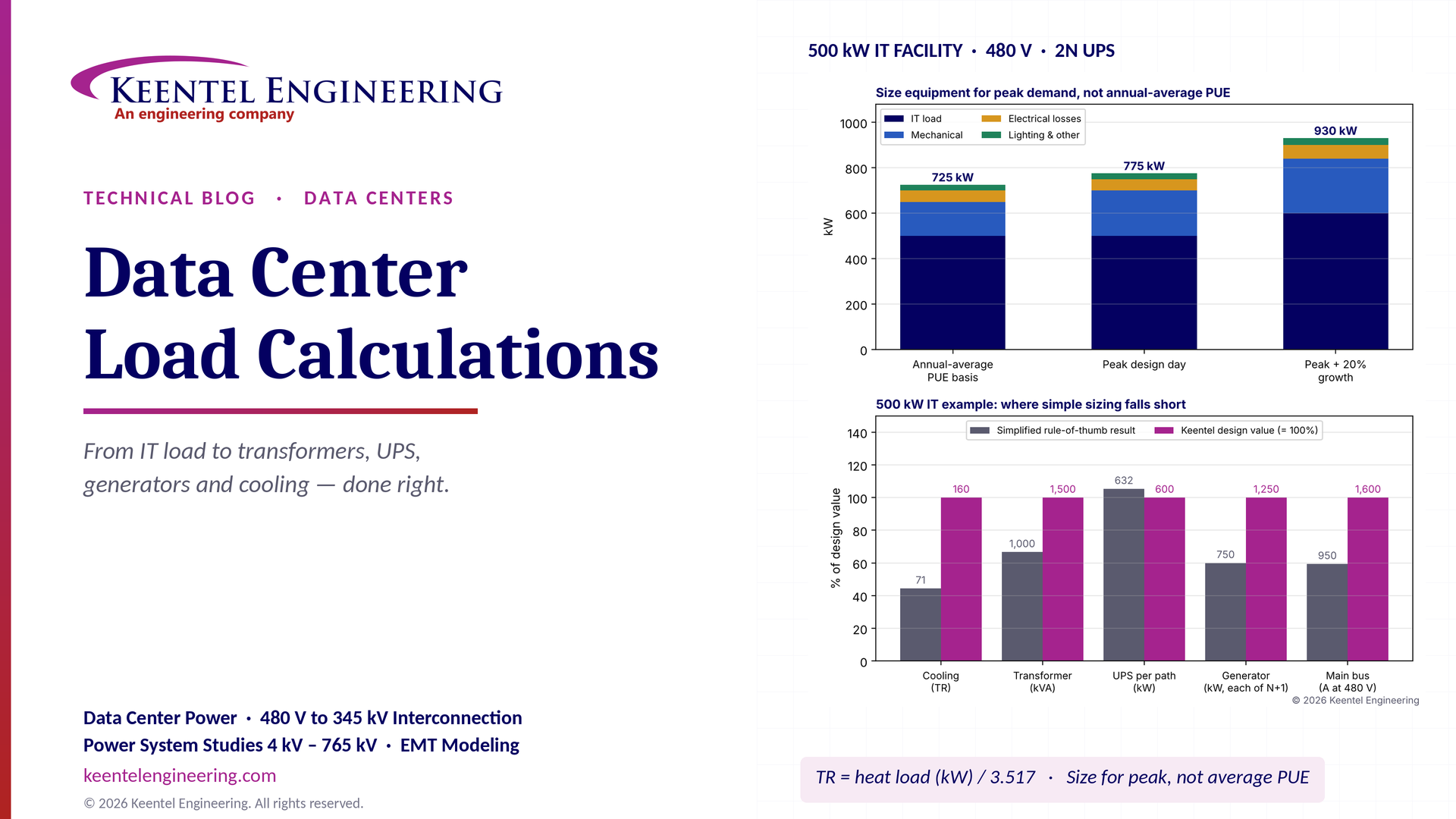
Learn data center electrical load calculations, including IT demand, PUE, UPS and generator sizing, cooling loads, redundancy, and worked US examples.
By SANDIP R PATEL
•
October 20, 2026
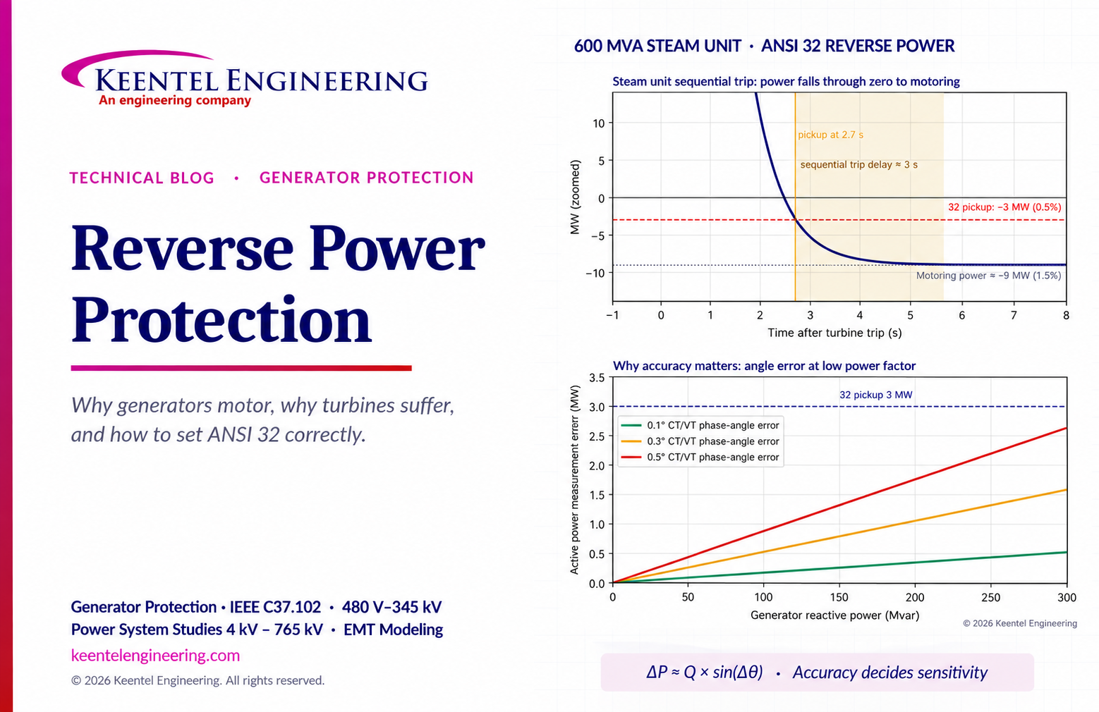
Learn reverse power protection (ANSI 32), generator motoring, relay pickup settings, time delays, sequential tripping and testing for US power plants.
Copy
By Team 2 Dexora
•
October 20, 2026
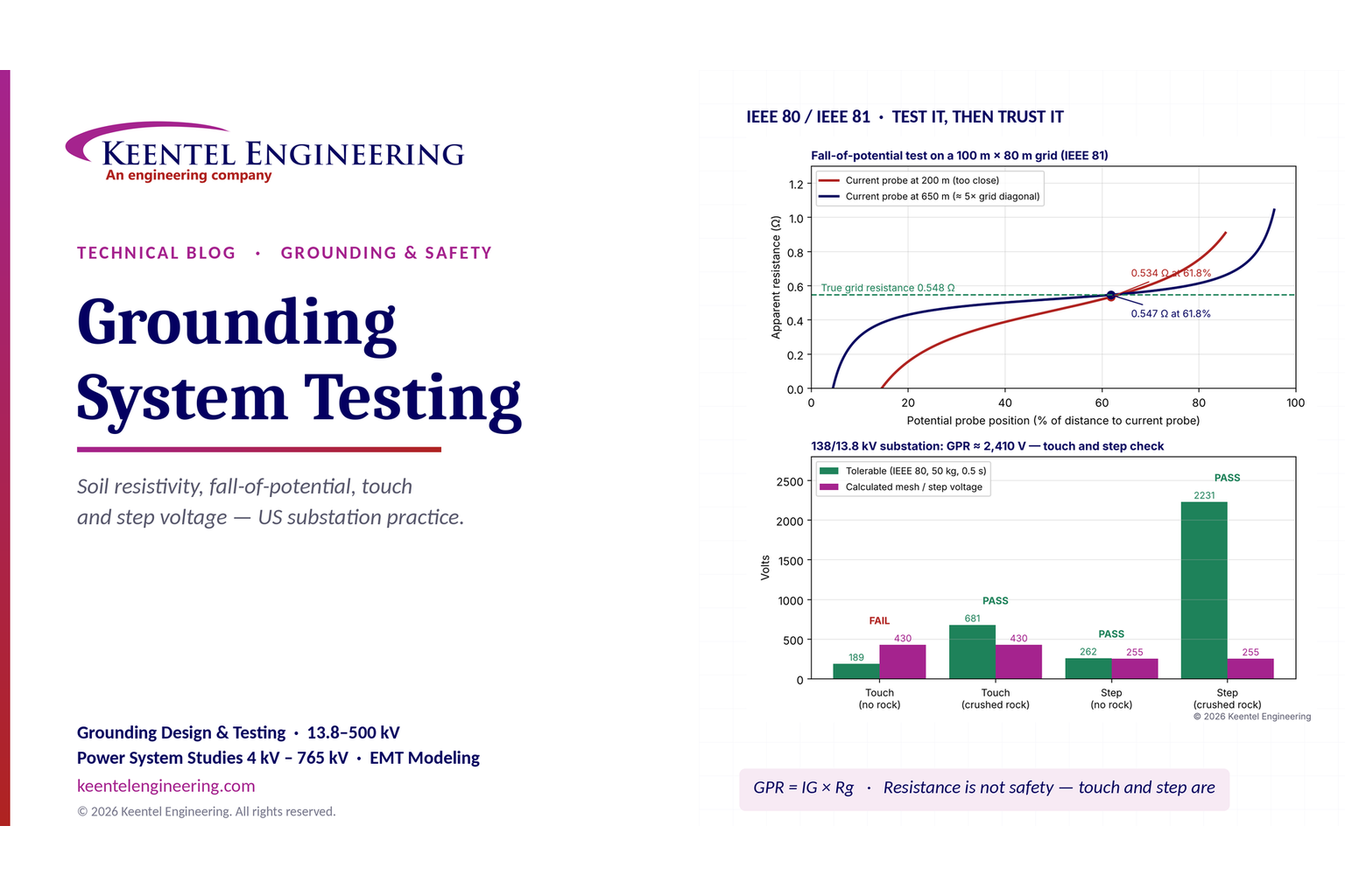
Explore grounding system testing with Keentel Engineering. Learn IEEE 80/81 methods, soil resistivity, ground resistance, and touch and step voltage safety.
By SANDIP R PATEL
•
October 13, 2026
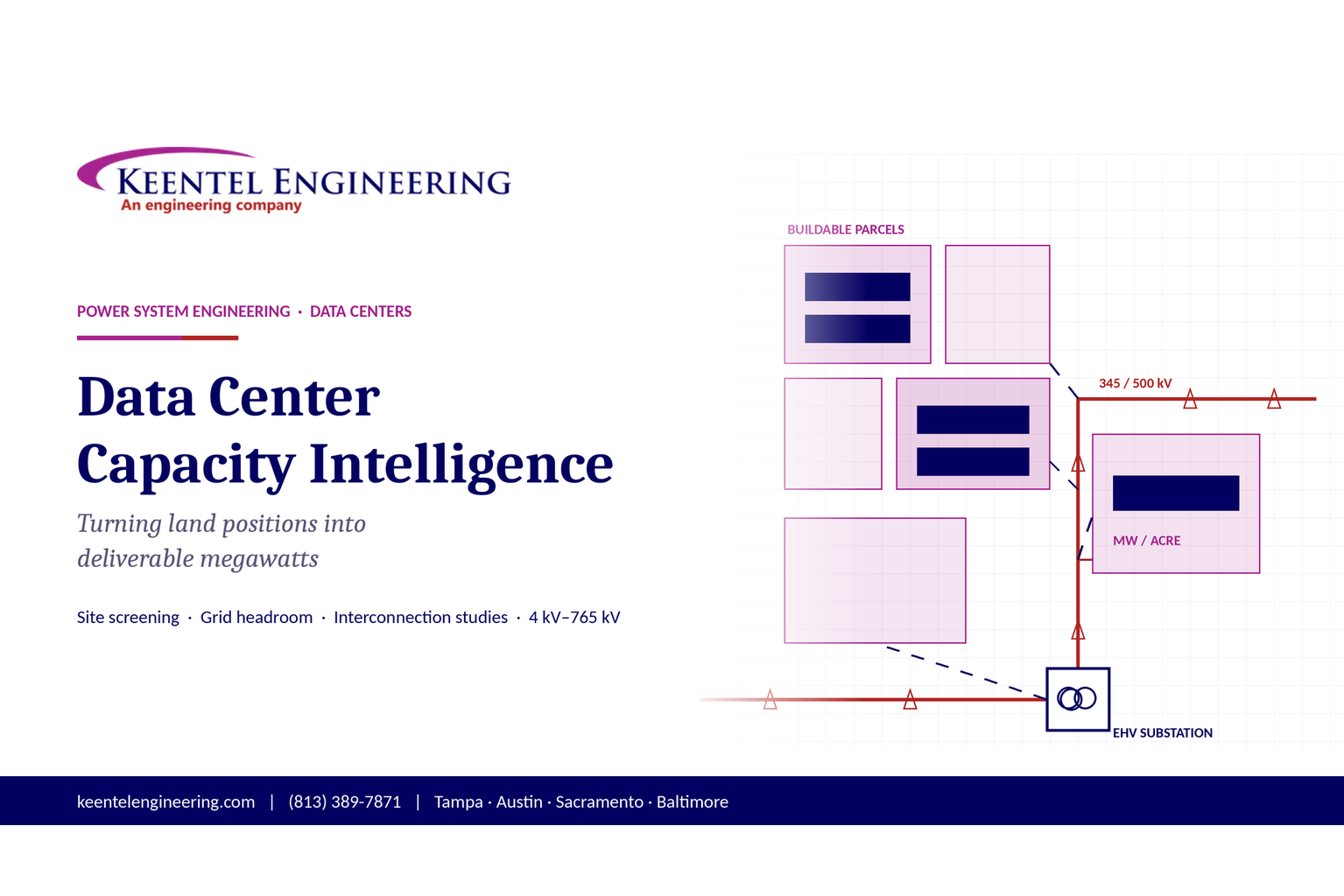
Plan data center capacity with land screening, MW-per-acre estimates, grid power availability and interconnection feasibility studies from Keentel Engineering.
By SANDIP R PATEL
•
October 11, 2026
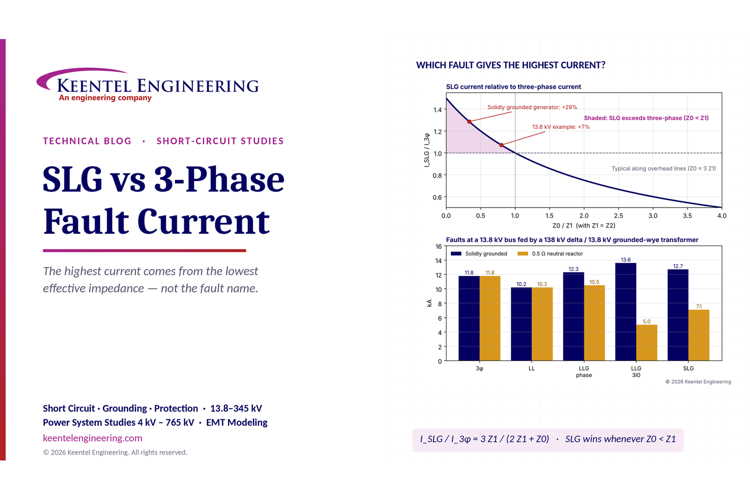
Learn which fault produces the highest current at a bus, why SLG faults can exceed three-phase faults, and how symmetrical components determine fault duty.
By SANDIP R PATEL
•
October 11, 2026
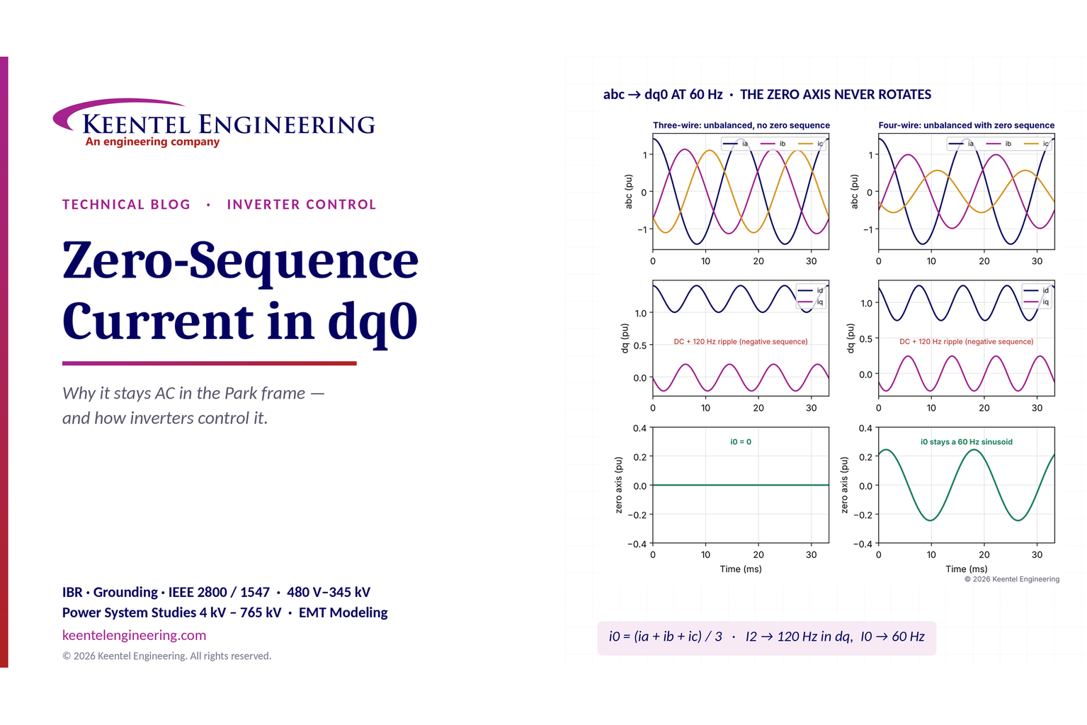
Learn why zero-sequence current pulsates in the dq0 frame, how Park's transformation works, and how inverter controls handle unbalance and ground faults.
By SANDIP R PATEL
•
October 11, 2026
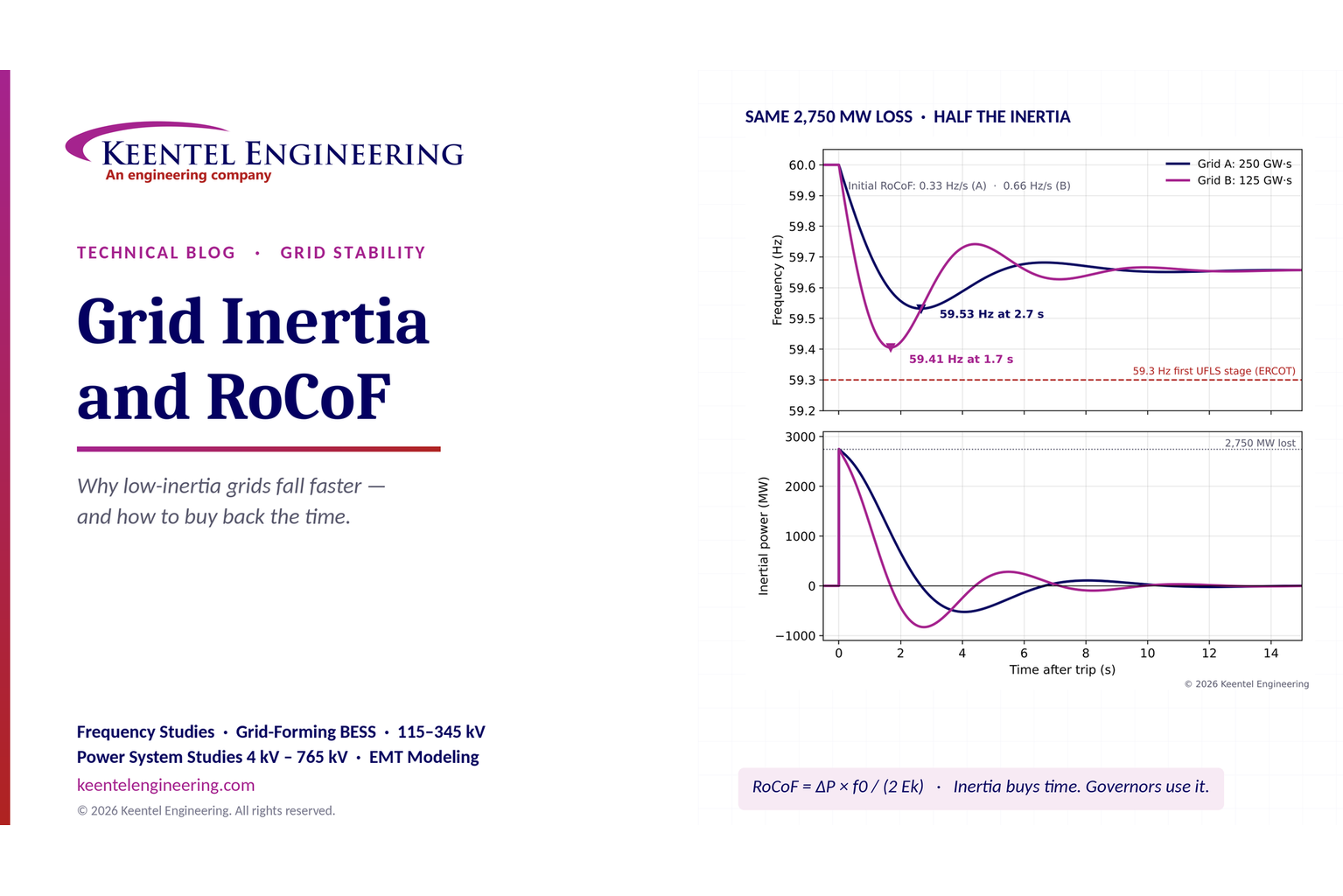
Explore grid inertia, RoCoF and frequency response, with swing equation calculations, frequency nadir analysis and US power system simulation examples.