A Coordinated Electric System Interconnection Review—the utility’s deep-dive on technical and cost impacts of your project.
Challenge: Frequent false tripping using conventional electromechanical relays
Solution: SEL-487E integration with multi-terminal differential protection and dynamic inrush restraint
Result: 90% reduction in false trips, saving over $250,000 in downtime
The three operating regions you have to design to
| Device | Output vs voltage | Response | Best suited to | Main limitations |
|---|---|---|---|---|
| Mechanically switched capacitor or reactor | Proportional to voltage squared | Seconds; discrete steps; limited switching operations per day | Steady-state reactive supply, voltage profile, loss reduction | No dynamic capability; step voltage change on switching; capability collapses when most needed |
| Static var compensator | Capacitive branches proportional to voltage squared | A few cycles; continuously controllable | Continuous control where cost matters and deep voltage support is not the driver | Square-law capability loss; harmonic filters are part of the plant and interact with the network |
| STATCOM | Approximately proportional to voltage — constant current capability | One to two cycles closed loop; converter response faster still | Voltage stability margin, weak interconnections, fast disturbance recovery, flicker and unbalance compensation | Higher capital cost; converter losses; adds a converter and its control dynamics to the network |
| Synchronous condenser | Governed by machine capability and excitation | Excitation response in the hundreds of milliseconds; inherent inertial response instantaneous | System strength and inertia, short-circuit contribution, black start support | Rotating plant with maintenance and losses; slower controlled response than a converter |
| STATCOM with energy storage | Reactive as a STATCOM, plus real power within the storage rating | As STATCOM for reactive; real power limited by storage | Where a real power deficiency is part of the problem | Cost and complexity of the storage; different failure and maintenance profile |
| Stage | Keentel scope | Outcome |
|---|---|---|
| Screening | Series-compensation proximity, radial contingency review, UIF and short-circuit ratio screening, frequency scans | Early identification of which SSO types apply |
| Detailed studies | PSCAD/EMTDC EMT studies with vendor real-code models, impedance-based and frequency-scan analysis | Clear evidence of stability margins or risk |
| Model quality | EMT model review, benchmarking against positive-sequence models, model acceptance support | Models that system operators accept |
| Mitigation | Control retuning recommendations with vendors, SSDC and bypass logic requirements, protection and monitoring specifications | Practical, coordinated solutions |
| Interconnection support | SSR and SSO study reports for ISO and utility requirements, response to reviewer comments | Fewer delays in the interconnection process |
Resilience: designing CDUs to the facility Tier objective
Liquid cooling makes heat removal more critical, not less. Cold plates hold only seconds of thermal buffer. If TCS flow stops, processors throttle or shut down very quickly. Resilience design must therefore cover:
- Pump redundancy: N+1 pumps at minimum, with automatic changeover.
- CDU redundancy: N+1 CDUs on a common TCS header, or 2N CDUs serving A and B manifolds for fault-tolerant designs.
- Power to CDUs: dual-corded CDUs fed from A and B sources, with pumps and controls on UPS power so coolant keeps flowing through a utility failure and generator start. This is the liquid-cooling equivalent of continuous cooling.
- Facility water continuity: chilled water or condenser water must also continue, through thermal storage, UPS-backed pumps or a high enough FWS temperature that the TCS can coast on stored thermal mass for the transfer period.
- Concurrent maintainability: isolation valves so any CDU, pump, filter or manifold section can be serviced without stopping the others.
- Leak management: leak detection, drip trays, automatic isolation valves and procedures for fluid spills.
Electrical engineering considerations
CDUs and liquid-cooling plants are electrical loads with their own design requirements:
- Pump motors and VFDs. Large CDUs use variable-frequency drives on their pump motors. These introduce harmonic current that must be included in the facility's harmonic study and IEEE 519 evaluation.
- Critical mechanical load on UPS. Putting CDU pumps on UPS increases UPS and battery sizing. The mechanical UPS load must be included in redundancy and ride-through calculations.
- Feeder and protection design. Dual feeds, automatic transfer, selective coordination and arc-flash labelling apply to CDU power distribution just as they do to IT power.
- Generator transient response. CDU pumps restarting together after a transfer create motor inrush on the generators. Staged restarts and soft acceleration reduce the step load.
- Load dynamics. AI training loads can swing rapidly between high and low power. Cooling controls must track those swings without temperature overshoot, and electrical systems must handle both the IT and the cooling load changes.
Commissioning a liquid-cooled data hall
- Flush and clean the TCS piping and manifolds to the specified cleanliness, using high-purity flush water.
- Fill and vent with the specified coolant, verifying glycol concentration and chemistry.
- Pressure test for leaks at design and test pressures, including quick-disconnect fittings.
- Verify sensors and controls: flow meters, temperature sensors, pressure transmitters, leak detection and BMS points.
- Load test with heat load banks connected through the cold-plate interfaces or rack manifolds, across the operating range.
- Prove the heat balance on both loops at several load steps, and the approach temperature against the design.
- Test failure scenarios: pump failure, CDU failure, power transfer to generator, valve failure and loss of facility water, confirming temperatures stay within the IT vendor's limits.
How Keentel Engineering helps
Keentel Engineering supports data center owners, developers and EPCs with the electrical engineering that liquid-cooled facilities depend on, and coordinates with the mechanical engineer of record and cooling vendors on the integrated design.
Transient Stability Analysis: An Engineering Guide for US Power Plants, Transmission Systems and Industrial Microgrids
October 11, 2026 | Blog
Part A — Transient Stability at a Glance
Every synchronous generator connected to the US grid — from a 13.8 kV cogeneration unit at an industrial plant to a 1,300 MVA nuclear unit feeding a 500 kV switchyard — spins in lockstep with every other synchronous machine in its interconnection. In normal operation, the mechanical power delivered by each turbine equals the electrical power the generator sends to the network, and the rotor holds a steady angle relative to the rest of the system. A severe disturbance breaks that balance. During a nearby short circuit, the generator can no longer deliver its electrical power, but the turbine keeps pushing. The rotor accelerates, its angle advances, and the question becomes simple and unforgiving: when protection clears the fault, will the network be able to pull the rotor back, or will the generator slip a pole and lose synchronism?
Transient stability analysis answers that question. It is one of the core power system studies behind every generator interconnection, every transmission plan, every protection scheme for a large plant and every industrial or data center microgrid that can island from the utility.
What a transient stability study evaluates
| Question | What the study determines | Why it matters |
|---|---|---|
| Do generators stay in synchronism after a large disturbance? | Rotor angle response of every machine | Loss of synchronism trips generators and can cascade |
| How fast must faults be cleared? | Critical clearing time (CCT) and stability margin | Sets breaker, relay and communication requirements |
| How do speed, angle, voltage and power behave? | Time-domain response for 10 to 20 seconds | Confirms damping, voltage recovery and frequency response |
| Which contingencies are critical? | Ranking of faults, outages and operating conditions | Focuses mitigation where it matters |
| Does protection perform correctly? | Relay and breaker timing, power swing response | Avoids unnecessary trips and missed trips |
| What happens if the plant islands? | Frequency, voltage and machine response after separation | Required for industrial, data center and campus microgrids |
The core relationships
- Swing equation: rotor acceleration is proportional to the difference between mechanical input power and electrical output power.
- Power-angle relationship: in the classical model, electrical power transfer equals E′V ÷ X × sin δ.
- Equal-area criterion: a single machine remains stable if the decelerating energy available after clearing is at least as large as the accelerating energy gained during the fault.
- Critical clearing time: the longest fault duration for which the system remains stable for a given operating condition and disturbance.
Keentel's worked example in one table
Keentel Engineering analyzed a 600 MVA generating unit delivering 540 MW through a step-up transformer and a 345 kV double-circuit line to a strong system. A bolted three-phase fault at the plant's 345 kV bus is cleared by tripping one circuit.
| Result | Value |
|---|---|
| Pre-fault rotor angle | 35.5° |
| Critical clearing angle (equal-area criterion) | 53.9° |
| Critical clearing time | 0.123 s, about 7.4 cycles |
| First swing peak, cleared in 4 cycles | 80° — stable with large margin |
| First swing peak, cleared in 7 cycles | 115° — stable with small margin |
| Cleared in 8 cycles | Loses synchronism |
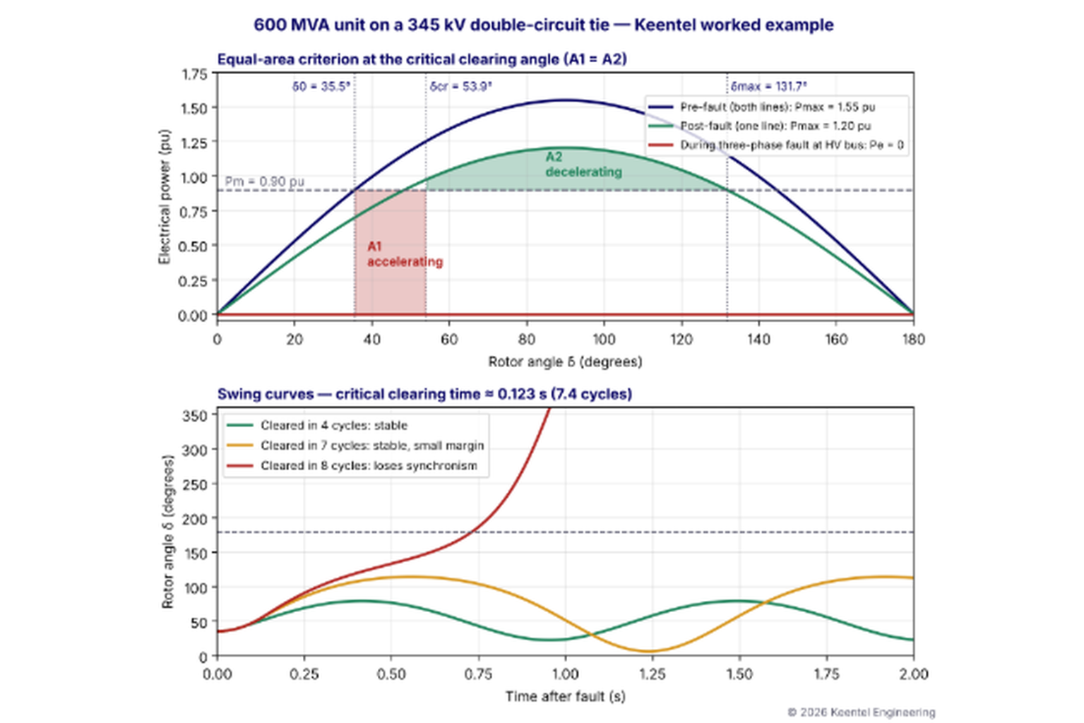
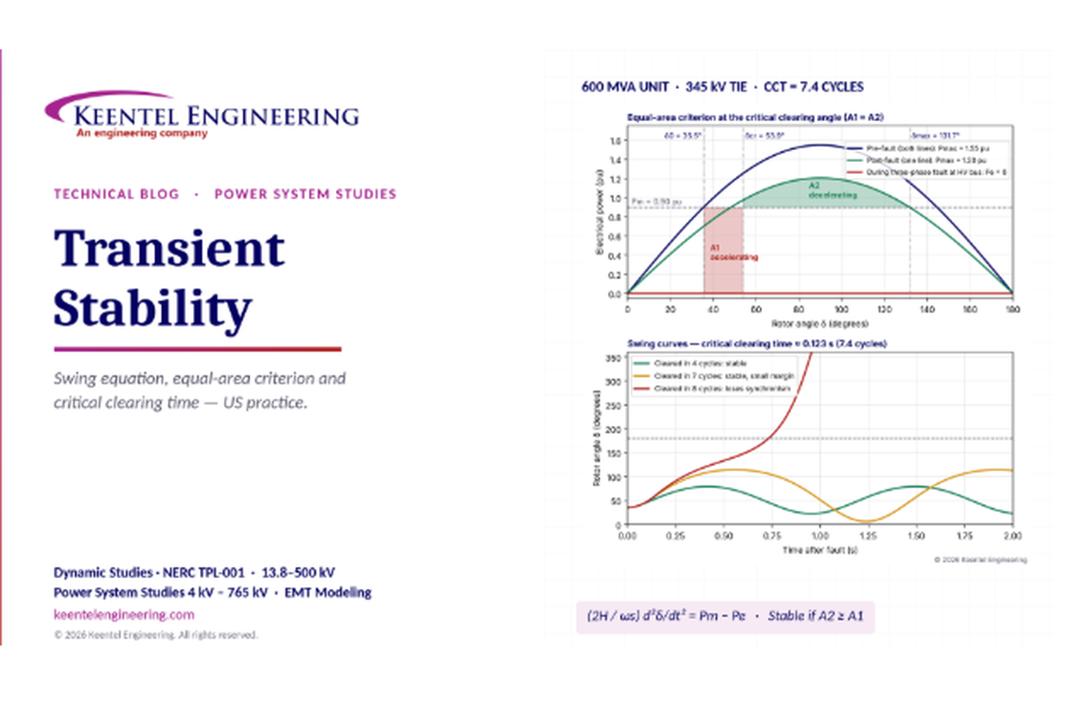
Figure 1. Top: power-angle curves before, during and after the fault, with accelerating area A1 and decelerating area A2 at the critical clearing angle. Bottom: rotor angle swing curves for clearing in 4, 7 and 8 cycles.
Transient stability is not just about whether a fault can be cleared. It is about whether the power system can withstand the disturbance and keep every generator in synchronism afterward.
Part B — Transient Stability Analysis: An Engineering Guide for US Power Plants, Transmission Systems and Industrial Microgrids
1. Where transient stability fits in power system stability
Power system stability is the ability of an electric power system, for a given initial operating condition, to regain a state of operating equilibrium after a physical disturbance, with most system variables bounded so that practically the entire system remains intact. The IEEE/CIGRE classification, first published in 2004 and extended in 2021 to address inverter-based resources, divides stability into several categories:
| Category | Sub-category | Time frame | Typical driver |
|---|---|---|---|
| Rotor angle stability | Small-disturbance (small-signal) | 10 to 20 s | Poorly damped electromechanical oscillations, 0.1 to 2 Hz |
| Rotor angle stability | Large-disturbance (transient) | 3 to 5 s, extended to 10 to 20 s for multi-swing behavior | Faults, line and generator trips |
| Voltage stability | Short-term and long-term | Seconds to minutes | Motor loads, tap changers, reactive limits |
| Frequency stability | Short-term and long-term | Seconds to minutes | Generation-load imbalance |
| Resonance stability | Electrical and torsional | Milliseconds to seconds | Subsynchronous resonance, torsional interaction |
| Converter-driven stability | Fast and slow interaction | Milliseconds to seconds | Inverter control interactions with the network |
Transient stability is the large-disturbance form of rotor angle stability. It asks whether synchronous machines keep their synchronism after a severe event such as a short circuit on a transmission line, loss of a large generator or loss of a major transmission element. Instability usually appears as aperiodic angle separation during the first swing, typically within one to two seconds. It can also appear on later swings when several modes of oscillation combine or when damping is poor, which is why US planning studies normally simulate at least 10 to 20 seconds after the disturbance.
In practice, a single transient stability study examines more than rotor angles. Modern planning criteria require engineers to verify voltage recovery, frequency response, damping, generator and inverter ride-through and relay performance in the same simulations. A plant that keeps synchronism but leaves voltage depressed for several seconds, or trips an adjacent inverter-based plant, has not passed a modern stability assessment.
2. The swing equation
2.1 Derivation from Newton's second law
A synchronous generator rotor and its turbine form a rigid rotating mass with moment of inertia J. The net accelerating torque equals the mechanical torque from the turbine minus the electromagnetic torque from the generator:
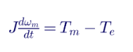
Multiplying by rotor speed converts torques into powers. Normalizing to the machine rating introduces the inertia constant H, defined as the stored kinetic energy at synchronous speed divided by the machine's MVA rating:
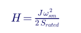
Expressing the rotor position as the electrical angle δ relative to a synchronously rotating reference gives the familiar per-unit swing equation:
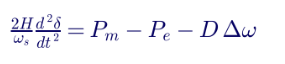
where H is in seconds on the machine base, ωs is synchronous electrical speed (2π × 60 = 377 rad/s in the US), δ is in electrical radians, Pm and Pe are mechanical and electrical power in per unit, and D represents damping from damper windings, loads and controls.
The form shown without a damping term — 2H/ωs × d²δ/dt² = Pm − Pe — is the classical swing equation. It is correct for first-swing analysis but omits damping, so it cannot by itself show whether oscillations decay after the first swing.
2.2 Practical checks on units
| Quantity | US value or convention | Common mistake |
|---|---|---|
| ωs | 377 rad/s electrical (60 Hz) | Using 314 rad/s (50 Hz) or mechanical speed |
| δ | Electrical radians in the equation; degrees for presentation | Mixing degrees and radians in the integration |
| H | Seconds on the machine MVA base | Using H on a different system base without conversion |
| M (inertia coefficient) | M = 2H/ωs in per-unit power · s²/rad | Confusing M with J |
| Speed deviation | Δω = dδ/dt, rad/s; often shown as Δf in Hz or slip in pu | Reporting slip without stating base |
When machines are combined or converted to a common system base, the inertia constant scales with rating:

2.3 Typical inertia constants
| Machine | Typical H (s, on machine MVA) |
|---|---|
| Large steam turbine-generator, 2-pole (fossil, nuclear) | 3 to 6 |
| Combustion turbine-generator | 4 to 9 |
| Combined-cycle steam turbine | 3 to 5 |
| Hydro generator (slow speed, salient pole) | 2 to 4 |
| Industrial gas or steam cogeneration unit | 2 to 5 |
| Reciprocating engine-generator | 0.5 to 2 |
| Synchronous condenser | 1 to 2, higher with flywheel |
| Large induction motors (for load modeling) | 0.3 to 1.5 |
Higher inertia slows the rotor's response, which gives protection more time. A reciprocating engine plant with H below 1 s can lose synchronism several times faster than a large steam unit for the same per-unit disturbance one reason industrial microgrids often need much faster clearing than utility transmission.
3. The power-angle relationship
3.1 The classical model
The classical model represents the generator as a constant voltage E′ behind its direct-axis transient reactance X′d, connected through a network reactance to an infinite bus of voltage V. Neglecting resistance, electrical power is:
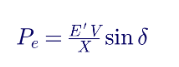
where X is the total transfer reactance between the internal voltage and the infinite bus. Maximum power occurs at δ = 90°:
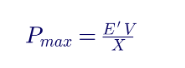
3.2 Where the classical model is not enough
The simple sin δ curve with a 90° peak is a useful teaching tool, but real studies must go further:
- Salient-pole machines: hydro generators have different direct- and quadrature-axis reactances. A reluctance term adds a sin 2δ component, and the peak occurs below 90°.
- Flux decay and excitation: E′ is not truly constant. Fast static exciters can raise field voltage during a fault and increase post-fault power transfer; slow exciters allow E′ to decay.
- Network losses and loads: resistance and loads shift the curve and the peak angle.
- Multi-machine systems: what matters is the angle between groups of machines, not the angle to an ideal infinite bus.
- Governor response: mechanical power is not exactly constant over several seconds.
For this reason, US planning studies use detailed generator models (GENROU, GENSAL and GENTPJ in PSS®E and PSLF), excitation system models from IEEE Std 421.5, governor models and power system stabilizer models, all validated under NERC MOD-026 and MOD-027 requirements.
4. The equal-area criterion
4.1 The principle
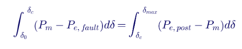
For a single machine connected to an infinite bus, multiplying the swing equation by dδ/dt and integrating gives a powerful result. The rotor returns toward equilibrium only if the energy it gains while accelerating can be removed while it decelerates. Graphically, on the power-angle diagram:
- Accelerating area A1: between the mechanical power line and the during-fault power curve, from the initial angle δ0 to the clearing angle δc.
- Decelerating area A2: between the post-fault power curve and the mechanical power line, from δc to the maximum angle the rotor reaches.
The system is stable if the available decelerating area is at least as large as the accelerating area:
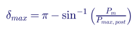
The largest possible decelerating area ends at δmax, where the post-fault curve crosses the mechanical power line again on its falling side:
4.2 Critical clearing angle
Solving the equal-area condition at the limit gives the critical clearing angle. When the during-fault and post-fault maximum powers are r1 and r2 times the pre-fault maximum Pmax:

4.3 Critical clearing time
For a bolted three-phase fault at the generator's high-voltage bus, electrical power during the fault is zero (r1 = 0), and the swing equation can be integrated directly. The rotor angle grows quadratically with time:
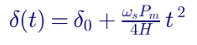
so the critical clearing time is:
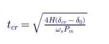
For any other fault a fault partway down a line, an unbalanced fault, or a fault with power still flowing there is no closed-form solution, and the critical clearing time is found by numerical simulation.
5. Worked example: a 600 MVA unit on a 345 kV double-circuit line
5.1 System data
| Element | Data (per unit on 600 MVA) |
|---|---|
| Generator | 600 MVA, 22 kV, 2-pole steam unit, X′d = 0.30, H = 4.0 s |
| Generator step-up transformer | 600 MVA, 22/345 kV, X = 0.15 |
| 345 kV transmission | Double-circuit line, X = 0.40 per circuit |
| System equivalent | X = 0.05, infinite bus at 1.0 pu |
| Operating point | P = 0.90 pu (540 MW), generator terminal voltage 1.0 pu |
| Disturbance | Bolted three-phase fault at the plant's 345 kV bus on one circuit, cleared by tripping that circuit |
5.2 Step 1: pre-fault conditions
The pre-fault external reactance, with both circuits in parallel, is 0.15 + 0.20 + 0.05 = 0.40 pu. Solving the load flow for 540 MW at 1.0 pu terminal voltage gives a generator reactive output of about 0.17 pu (100 Mvar) and a stator current of 0.92 pu. The internal voltage behind transient reactance is:
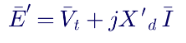
giving E′ = 1.084 pu at an angle of 35.5° relative to the infinite bus.
| Network condition | Transfer reactance X (pu) | Pmax = E′V/X (pu) |
|---|---|---|
| Pre-fault, both circuits | 0.30 + 0.40 = 0.70 | 1.55 |
| During fault at 345 kV bus | Infinite (bus voltage zero) | 0 |
| Post-fault, one circuit | 0.30 + 0.15 + 0.40 + 0.05 = 0.90 | 1.20 |
The pre-fault angle confirms the operating point: δ0 = sin⁻¹(0.90 ÷ 1.55) = 35.5°.
5.3 Step 2: maximum angle and critical clearing angle
With post-fault Pmax = 1.20 pu:
- δmax = 180° − sin⁻¹(0.90 ÷ 1.20) = 131.7°
- r1 = 0 and r2 = 1.20 ÷ 1.55 = 0.78
Applying the critical clearing angle equation (or equivalently setting A1 = A2 directly on the post-fault curve) gives δcr = 53.9°.
The accelerating area at the limit is Pm × (δcr − δ0) = 0.90 × 0.321 rad = 0.289 pu·rad, matched exactly by the decelerating area under the post-fault curve between 53.9° and 131.7°.
5.4 Step 3: critical clearing time

The critical clearing time is 0.123 s, or 7.4 cycles at 60 Hz. Keentel's numerical integration of the swing equation gives the same result to within 0.1 ms, confirming the analytical method.
5.5 Step 4: what the clearing time means
| Total clearing time | Rotor angle at clearing | Slip at clearing | First swing peak | Result |
|---|---|---|---|---|
| 3 cycles | 38.6° | 0.34 Hz | 73° | Stable, large margin |
| 4 cycles | 40.9° | 0.45 Hz | 80° | Stable, large margin |
| 5 cycles | 44.0° | 0.56 Hz | 88° | Stable |
| 6 cycles | 47.7° | 0.68 Hz | 99° | Stable |
| 7 cycles | 52.1° | 0.79 Hz | 115° | Stable, small margin |
| 8 cycles | 57.2° | 0.90 Hz | Unbounded | Loses synchronism |
Modern 345 kV protection with communication-assisted tripping and 2- or 3-cycle breakers typically clears faults in about 3.5 to 5 cycles, so this unit is stable for normal clearing. But if a breaker fails and breaker failure protection must trip adjacent breakers, total clearing time often reaches 10 to 15 cycles — beyond the 7.4-cycle limit. That delayed-clearing event, required by NERC TPL-001, would drive design changes such as faster breaker failure schemes, independent pole tripping, power system stabilizer tuning or a lower operating limit.
5.6 Sensitivity to inertia and loading
| Case | Critical clearing time |
|---|---|
| Base case: H = 4.0 s, P = 0.90 pu | 7.4 cycles |
| H = 3.0 s | 6.4 cycles |
| H = 6.0 s | 9.1 cycles |
| P = 0.70 pu | 12.1 cycles |
| P = 0.80 pu | 9.6 cycles |
| P = 1.00 pu | 5.3 cycles |
Two conclusions follow. First, CCT is much more sensitive to loading than to inertia: increasing output from 90% to 100% cuts the clearing time margin by almost 30%. Second, critical clearing time is not a property of the generator alone; it belongs to a specific operating condition, network topology and disturbance.
5.7 Fault location matters
If the same three-phase fault occurs at the middle of one 345 kV circuit instead of at the plant bus, some power still flows during the fault. The during-fault transfer reactance rises to 2.35 pu, so the during-fault Pmax is about 0.46 pu instead of zero. Keentel's simulation gives a critical clearing time of about 0.185 s, or 11.1 cycles — 50% longer than for the close-in fault. That is why stability studies always include close-in faults at the plant's high-voltage bus: they are usually the most severe.
6. What happens during and after a fault
The sequence of events follows four stages:
| Stage | Electrical condition | Rotor behavior |
|---|---|---|
| 1. Before the fault | Pm = Pe; steady angle | Rotor at synchronous speed |
| 2. During the fault | Pe falls sharply, often close to zero for close-in three-phase faults; Pm nearly constant | Rotor accelerates; angle increases |
| 3. After clearing | Pe jumps up on the post-fault curve, above Pm | Rotor decelerates but angle continues to increase until speed returns to synchronous |
| 4. Recovery | Oscillations around the new equilibrium | Damped by damper windings, excitation, PSS and loads; synchronism restored if stable |
Three points are often overlooked:
- The angle keeps increasing after clearing. The rotor is above synchronous speed when the fault clears, so the angle continues to advance until the decelerating energy brings speed back to synchronous. The maximum angle occurs after clearing, not at clearing.
- Unbalanced faults are less severe. Single-line-to-ground faults leave two phases transferring power, so less acceleration occurs. Three-phase faults are typically the design basis for normal clearing; single-line-to-ground faults are often the design basis for delayed clearing in planning criteria.
- Mechanical power is not instantaneously constant. Steam and gas turbine governors respond within seconds; fast valving can reduce mechanical power within a fraction of a second on some steam units, improving stability.
7. Multi-machine systems
Real interconnections contain thousands of machines. For multi-machine systems, stability depends on whether groups of machines separate from each other. Engineers examine:
- Relative rotor angles: the spread between the most advanced and least advanced machine angles, commonly referenced to a center-of-inertia angle.
- Coherent groups: machines that swing together, such as all units at one plant or in one region.
- Inter-area modes: groups of machines in different regions oscillating against each other at 0.1 to 0.8 Hz.
- Local plant modes: a plant oscillating against the rest of the system at roughly 0.8 to 2 Hz.
The center-of-inertia angle is:
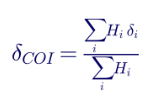
Commonly used screening criteria flag instability when relative rotor angles exceed about 180° or when angles diverge without bound. Utilities and planning coordinators also apply damping criteria, such as requiring oscillations to decay to a defined percentage within a set time, and voltage recovery criteria.
8. Modeling for US transient stability studies
8.1 Generator models
| Model (PSS®E/PSLF naming) | Application |
|---|---|
| GENCLS | Classical model; screening and distant equivalents only |
| GENROU / GENROE | Round-rotor machines (steam and gas turbine generators), subtransient detail |
| GENSAL / GENSAE | Salient-pole machines (hydro) |
| GENTPJ / GENQEC | Models with improved saturation representation |
8.2 Controls
- Excitation systems: static and brushless exciters represented by IEEE Std 421.5 models such as ST4C, ESST1A, AC7B and EXST1, with their limiters.
- Power system stabilizers: PSS2A, PSS2B and PSS2C models add damping to electromechanical oscillations. Many US utilities and regions require PSS on large units.
- Governors and turbines: steam, gas turbine and hydro governor models such as IEEEG1, GGOV1 and HYGOV, with deadbands and droop consistent with FERC Order No. 842 requirements for new resources.
- Inverter-based resources: WECC generic models (REGC, REEC and REPC) in positive-sequence studies, and vendor-specific models in EMT studies.
8.3 Loads
Loads strongly affect transient stability. Composite load models represent induction motors that slow down and stall during faults, drawing high reactive current and depressing voltage. Static constant-impedance load assumptions can produce optimistic results.
8.4 Protection
Relays that may operate during the simulation must be represented: distance relays that could trip on stable swings, generator out-of-step relays, under- and over-frequency and voltage relays, and IBR ride-through settings. NERC PRC-026 requires owners of certain elements to evaluate whether their relays could trip on stable power swings identified in planning studies.
8.5 Model validation
Model quality determines study quality. NERC MOD-026 (verification of excitation and voltage control models) and MOD-027 (verification of turbine-governor and active power models), and the successor standard developed to consolidate them, require generator owners to provide models validated against measured data. Event playback using PMU and DFR recordings is increasingly used to confirm model accuracy.
9. Positive-sequence RMS versus EMT simulation
| Feature | RMS (positive-sequence) simulation | EMT simulation |
|---|---|---|
| Tools | PSS®E, PSLF, PowerWorld, PowerFactory RMS | PSCAD, EMTP, PowerFactory EMT |
| Time step | About a quarter to half cycle | Microseconds |
| Network | Phasor, fundamental frequency | Instantaneous three-phase waveforms |
| System size | Entire interconnection | Local area, often with equivalents |
| Strengths | Large-system rotor angle, voltage and frequency stability | Weak grids, inverter controls, harmonics, unbalance, protection detail |
| Typical use | Interconnection and planning studies | IBR studies in low-SCR areas, FACTS and HVDC, detailed protection |
Classical transient stability problems involving synchronous machines are well suited to RMS simulation. As inverter-based resources replace synchronous generators, many US transmission providers require EMT studies alongside RMS studies, especially where short-circuit ratio is low.
10. US planning criteria and standards
10.1 NERC TPL-001
NERC TPL-001, Transmission System Planning Performance Requirements, defines the contingencies that planners must study and the performance required. Key categories include:
| Planning event | Description | Typical stability study case |
|---|---|---|
| P0 | System intact, no contingency | Base case |
| P1 | Single contingency: loss of a generator, transmission circuit, transformer, shunt device or single pole of DC, with normal clearing | Three-phase fault with normal clearing |
| P2 | Single event: opening of a line section without a fault, bus section fault, internal breaker fault | Bus and breaker faults |
| P3 | Loss of a generator followed by system adjustment and a second single contingency | Generator outage plus fault |
| P4 | Multiple contingencies caused by a fault plus stuck breaker | Delayed clearing by breaker failure protection |
| P5 | Multiple contingencies caused by a fault plus failure of a non-redundant protection component | Delayed clearing by remote backup |
| P6 | Two overlapping single contingencies | Prior outage plus fault |
| P7 | Common-structure contingency, such as loss of two circuits on a common tower | Double-circuit outage |
| Extreme events | Beyond the planning categories; evaluated for consequences | Severe events such as loss of a substation |
TPL-001 requires that generators remain stable and that voltage oscillations be adequately damped for the specified events, with performance requirements that differ by category. Many planning coordinators, ISOs and utilities add specific criteria for voltage recovery, damping and relay margin.
10.2 Other NERC and FERC requirements
- FAC-002: studies of new or materially modified facilities, including stability effects of generator and transmission interconnections.
- PRC-024 and PRC-029: generator and IBR frequency and voltage ride-through, which must be reflected in stability simulations.
- PRC-026: relay performance during stable power swings.
- PRC-019: coordination of generator voltage regulating controls, limiters and protection.
- MOD-032, MOD-026 and MOD-027: model data and model verification for planning studies.
- FERC Order No. 2023: interconnection process reforms affecting study timing, cluster studies and model requirements.
10.3 IEEE guidance
- IEEE Std 1110: guide for synchronous generator modeling practices in stability analyses.
- IEEE Std 421.5: excitation system models for power system stability studies.
- IEEE Std C37.102: guide for AC generator protection, including out-of-step (78) protection.
- IEEE Std 3002 series (successor to IEEE Std 399, the Brown Book): recommended practices for industrial and commercial power system analysis, including stability studies.
- IEEE PES Power System Relaying and Control Committee reports: power swing and out-of-step considerations for transmission protection.
11. Critical clearing time and protection design
11.1 Components of total clearing time
| Component | Typical time at 115 to 345 kV |
|---|---|
| Relay operating time | 0.5 to 1.5 cycles for high-speed elements |
| Communication-assisted scheme channel time | 0.25 to 1 cycle |
| Auxiliary relay time (if any) | 0.25 to 0.5 cycle |
| Breaker interrupting time | 2, 3 or 5 cycles depending on rating |
| Total normal clearing | About 3.5 to 6 cycles |
| Breaker failure timer plus backup breaker | 8 to 12 cycles additional delay in many schemes |
| Total delayed clearing (stuck breaker) | Commonly 10 to 15 cycles or more |
| Remote backup (zone 2 time delay) | 20 to 30 cycles or more |
11.2 Stability margin
A study should not stop at a yes/no answer for normal clearing. Engineers compare the actual clearing time with the critical clearing time:

For the worked example, normal clearing at 4 cycles gives about 46% margin, while a 12-cycle stuck-breaker case has negative margin and is unstable. Many utilities set minimum margins for critical plants, often expressed in cycles above the expected clearing time.
11.3 Out-of-step and power swing protection
When a generator loses synchronism, it slips poles and produces large current and torque pulsations that can damage the machine and shaft. Generator out-of-step protection (device 78) detects the apparent impedance trajectory crossing the generator and transformer and trips the unit, ideally at a favorable angle to limit breaker stress. On transmission lines, power swing blocking prevents distance relays from tripping on stable swings, while out-of-step tripping separates the system at planned locations if instability does occur. Settings must come from the same stability simulations, using the apparent impedance trajectories of stable and unstable swings.
12. Methods for improving transient stability
| Method | How it helps | Typical application |
|---|---|---|
| Faster fault clearing | Reduces accelerating area | Communication-assisted protection, 2-cycle breakers, faster breaker failure schemes |
| Independent pole operation | Reduces severity of stuck-breaker three-phase faults to single-phase | Large generator and EHV breakers |
| High initial response excitation | Raises internal voltage after the fault, increasing decelerating area | Static exciters with high ceiling voltage |
| Power system stabilizers | Damp swings after the first peak | Large synchronous units |
| Reduced transfer reactance | Raises Pmax | Additional circuits, series compensation, higher-voltage tie |
| Series compensation | Reduces line reactance | Long 345 kV and 500 kV lines, with subsynchronous resonance studies |
| Dynamic reactive support | Holds voltage, increasing power transfer | STATCOMs, SVCs, synchronous condensers |
| Fast valving | Reduces mechanical power during and after the fault | Selected steam units |
| Generator tripping or runback schemes | Removes accelerating power after critical contingencies | Remedial action schemes (RAS) under NERC PRC-012 |
| Braking resistors | Absorb accelerating energy | Rare, selected remote hydro plants |
| Operating limits | Reduce pre-fault loading | Interim measure when other options are not available |
13. Grid-connected versus islanded operation
Industrial plants, refineries,
data centers, universities and hospitals often own synchronous generators that run in parallel with the utility and may need to island during a disturbance. Their stability behaves very differently in the two modes:
| Factor | Grid-connected | Islanded |
|---|---|---|
| Frequency reference | Set by the interconnection | Set by local generators and their governors |
| Fault level | High, from the utility | Low, from local machines only |
| Voltage support | Strong | Limited to local excitation and reactive devices |
| Power imbalance | Absorbed by the grid | Must be balanced by local generation and load shedding |
| Rotor angle concern | Local plant swinging against the grid | Machines swinging against each other; frequency stability dominates |
| Protection | Utility-coordinated settings | Lower fault currents may require adaptive or separate settings |
13.1 Islanding studies
A study for a facility that can island typically evaluates:
- Separation detection: how the facility detects the grid event, using under-frequency, under-voltage, rate-of-change-of-frequency or transfer trip signals.
- Separation timing: how quickly the facility breaker opens, and whether local machines are still stable at that moment.
- Power balance after separation: if the facility was importing power, local generation must pick up the deficit or load must be shed.
- Frequency and voltage recovery: governor and excitation response, motor reacceleration and load shedding stages.
- Protection in island mode: reduced fault current may affect feeder and generator protection.
- Resynchronization: synchronizing checks (device 25) for reconnection to the utility.
13.2 Example: island separation from a 69 kV utility tie
A 40 MW industrial plant with two 25 MVA gas turbine generators at 13.8 kV imports 8 MW from a 69 kV utility tie. When a utility fault causes separation, the generators must instantly pick up the 8 MW import. With a combined H of about 4.5 s on 50 MVA, the initial rate of frequency decline is roughly:

Without fast load shedding, the plant frequency would reach typical generator under-frequency trip settings within a few seconds, depending on governor response. Studies define load shedding blocks and timing so frequency recovers before generator protection operates.
14. Inverter-based resources and transient stability
Solar, wind and battery storage connected through inverters are changing transient stability in four ways:
- Less synchronous inertia: fewer synchronous machines online means larger angle and frequency deviations for the same disturbance.
- Different fault response: IBRs supply limited, controlled fault current, roughly 1.0 to 1.5 times rated, and their active power during and after faults depends on control settings.
- Ride-through behavior: if IBRs reduce active power or trip during faults, synchronous machines nearby experience different accelerating power than in traditional studies.
- New stability forms: converter-driven stability and weak-grid interactions, which may require EMT studies.
IEEE 2800-2022 and NERC PRC-029 define ride-through and recovery requirements for transmission-connected IBRs. Transient stability studies for plants near large IBR concentrations must model these resources accurately, including active power recovery ramp rates after faults, which directly affect neighboring generators' rotor angle swings.
15. Practical study workflow
| Step | Activity | Output |
|---|---|---|
| 1 | Define scope, criteria, study area, contingency list and operating conditions | Study plan agreed with the transmission provider or owner |
| 2 | Build or obtain base cases: peak, off-peak, light load, high transfer | Load flow cases |
| 3 | Assemble dynamic data: generator, exciter, PSS, governor, IBR and load models | Validated dynamic database |
| 4 | Initialize and run a flat (no-disturbance) simulation | Confirmation that models are correctly initialized |
| 5 | Run contingencies: normal clearing, delayed clearing, multiple contingencies | Time-domain results |
| 6 | Evaluate rotor angles, speeds, voltages, frequency, damping and relay performance | Pass or fail against criteria |
| 7 | Determine critical clearing times for key faults | Stability margins |
| 8 | Develop and test mitigation | Recommended solutions |
| 9 | Document assumptions, results and recommendations | Study report |
| 10 | Validate after commissioning using measured data | Updated models |
15.1 Flat run and initialization checks
Every dynamic study should begin with a flat run of at least 10 to 20 seconds with no disturbance. All machine angles, speeds, voltages and controller outputs should remain constant. Drift usually indicates initialization errors, inconsistent data or controllers operating at limits.
15.2 Interpreting results
| Plot | What to look for |
|---|---|
| Rotor angles (relative to reference or COI) | Bounded first swing; decaying oscillations |
| Generator speed | Return to synchronous speed; no runaway |
| Bus voltages | Recovery to acceptable levels within the required time; no prolonged depression |
| Active and reactive power | Expected recovery; no sustained oscillation |
| Field voltage and limiters | Exciter response within limits |
| Apparent impedance at line and generator relays | Margin to relay characteristics for stable swings |
| Frequency | Nadir and recovery within criteria |
16. Common study pitfalls
- Using classical models for detailed studies: classical models omit excitation, saturation and damper effects and may give misleading results.
- Unvalidated or default data: typical parameters can differ significantly from the actual machine and control settings.
- Ignoring delayed clearing: normal clearing may pass, while stuck-breaker cases fail.
- Modeling loads as constant impedance: this can hide voltage recovery and motor stall problems.
- Leaving out protection: relays that trip during the event change the outcome.
- Studying only peak load: light-load, high-renewable or high-transfer cases may be more severe.
- Inadequate simulation length: some instabilities appear on the second or later swings.
- Ignoring IBR behavior: active power recovery and ride-through settings change neighboring generator swings.
17. Worked example 2: how fault type changes the critical clearing time
Planning criteria use different fault types for different events, so engineers need to know how much each type shortens or lengthens the clearing time limit. In positive-sequence stability programs, an unbalanced fault is represented by connecting a fault shunt at the faulted bus in the positive-sequence network. Its value comes from the negative- and zero-sequence Thevenin impedances at that bus:
| Fault type | Positive-sequence fault shunt |
|---|---|
| Three-phase | Zero (bolted short circuit) |
| Line-to-line | Z2 |
| Double line-to-ground | Z2 in parallel with Z0 |
| Single line-to-ground | Z2 + Z0 |
With a fault shunt Xf at the plant's 345 kV bus, the during-fault transfer reactance between the generator internal voltage and the system becomes:

where Xa is the reactance from the generator internal voltage to the faulted bus (X′d plus the step-up transformer, 0.45 pu) and Xb is the reactance from the bus to the system (two circuits in parallel plus the system equivalent, 0.25 pu). Taking Z2 equal to the positive-sequence Thevenin reactance at the bus (0.161 pu) and a zero-sequence Thevenin reactance of 0.10 pu, typical for a bus fed by a delta-wye grounded step-up transformer, Keentel's simulations give:
| Fault at 345 kV plant bus | Fault shunt Xf (pu) | During-fault transfer reactance (pu) | During-fault Pmax (pu) | Critical clearing time |
|---|---|---|---|---|
| Three-phase | 0 | Infinite | 0 | 7.4 cycles |
| Double line-to-ground | 0.062 | 2.53 | 0.43 | 10.7 cycles |
| Line-to-line | 0.161 | 1.40 | 0.78 | 17.7 cycles |
| Single line-to-ground | 0.261 | 1.13 | 0.96 | 33.1 cycles |
The single-line-to-ground fault allows more than four times the clearing time of the three-phase fault. This is why many planning criteria apply three-phase faults with normal clearing but single-line-to-ground faults for delayed-clearing events: a stuck breaker on a single-phase fault is far less severe. It is also why independent pole operation of breakers, which limits a stuck breaker to one phase, is such an effective stability measure at large generating stations.
18. Numerical integration in stability programs
Commercial stability programs solve thousands of nonlinear differential equations for machines, controls and loads, together with the algebraic network equations, at every time step. Two broad approaches are used:
| Method | Description | Characteristics |
|---|---|---|
| Explicit (for example, modified Euler or Runge-Kutta) | Calculates the next state from derivatives at the current step | Simple and fast per step; time step limited by the fastest model time constant |
| Implicit (for example, trapezoidal rule) | Solves the next state simultaneously with the network | Numerically stable with stiff models; larger time steps possible |
A typical positive-sequence time step is a quarter to half cycle (about 4 to 8 ms). Engineers should check that results do not change when the time step is halved, that fast controllers with very small time constants are not causing numerical instability, and that network switching events occur exactly at the intended times. Results that change with time step, or controllers that oscillate at the integration frequency, indicate model or data problems rather than physical behavior.
For the single-machine worked examples in this article, Keentel integrated the swing equation with a 0.1 ms step and confirmed the analytical critical clearing time to within 0.1 ms.
19. Direct methods and screening
Running every contingency at every operating point is time-consuming, so engineers use screening techniques to focus detailed simulation where it matters:
- Transient energy function (Lyapunov) methods: extend the equal-area concept to multi-machine systems by comparing the system's kinetic and potential energy at fault clearing with a critical energy value. They provide a stability margin directly but depend on simplified models.
- Extended equal-area criterion (SIME and related methods): reduce the multi-machine system to an equivalent one-machine system for the critical group of machines, combining time-domain results with equal-area insight.
- Contingency ranking: severity indices based on early rotor angle acceleration, kinetic energy at clearing or voltage dips rank contingencies before full simulation.
- Dynamic security assessment (DSA): online tools used by many US reliability coordinators and transmission operators run stability simulations on near-real-time cases to determine operating limits.
Screening methods guide the study, but final conclusions in US planning work rest on detailed time-domain simulation with validated models.
20. Voltage and frequency performance in stability studies
A transient stability study is judged by more than rotor angles. Planning coordinators and utilities apply additional performance criteria to the same simulations:
| Criterion | Typical form (varies by region and utility) | Purpose |
|---|---|---|
| Transient voltage recovery | Bus voltages recover above a specified level, such as 0.8 to 0.9 pu, within a specified time after clearing | Avoid motor stalling, load loss and IBR trips |
| Transient voltage dip duration | Limits on how long voltage may remain below thresholds | Protect customer equipment and ride-through compliance |
| Damping | Oscillations decay to a specified fraction within a specified time, or minimum damping ratio | Avoid sustained oscillations |
| Frequency | Frequency stays above under-frequency load shedding thresholds and recovers | Prevent load shedding and generator trips |
| Relay margin | Apparent impedance during stable swings stays outside relay trip zones by a defined margin | Prevent unintended line tripping (PRC-026) |
| Generator and IBR ride-through | No unintended tripping within PRC-024 and PRC-029 boundaries | Maintain generation during disturbances |
These criteria often reveal problems that rotor angle plots alone would miss. A plant that remains in synchronism but causes prolonged low voltage at a nearby load center, or causes neighboring inverter-based plants to enter momentary cessation, still requires mitigation.
21. Large loads, data centers and transient stability
The rapid growth of large loads in the US — hyperscale data centers, AI training campuses, cryptocurrency mining facilities, hydrogen electrolyzers and large industrial electrification projects — is introducing new transient stability considerations at 115 kV to 345 kV.
- Load loss as a disturbance: large power-electronic loads can disconnect or transfer to backup power during voltage dips. Loss of hundreds of megawatts of load in a fraction of a second causes over-frequency and can accelerate nearby generators. NERC has documented events in which large data center loads dropped offline during transmission faults.
- Fault ride-through of loads: unlike generators, large loads have historically had no ride-through requirements. Transmission providers increasingly ask large-load customers to specify and verify voltage ride-through behavior.
- On-site generation and islanding: campuses with on-site gas turbines, reciprocating engines or fuel cells must be studied for both grid-connected and islanded stability, including the transition between them.
- Rapid load fluctuations: AI training workloads can change power by large fractions of the facility rating within seconds, which can excite electromechanical modes and stress on-site generators' governors.
- Modeling: large loads require dynamic models that represent their power electronics, protection and ride-through behavior, rather than static load models.
Keentel Engineering studies these facilities with the same methods used for generators: time-domain simulation of faults, ride-through and islanding, with protection represented explicitly.
22. What a complete transient stability study report contains
A study is only as useful as its documentation. A complete report allows the transmission provider, owner and future engineers to understand, reproduce and rely on the results:
- Purpose and scope: the project, the questions the study answers and the applicable criteria.
- System representation: base cases, study area, operating conditions and future projects included.
- Dynamic data: generator, excitation, PSS, governor, IBR, load and protection models, with sources and validation status.
- Contingency list: each event with fault type, location, clearing times and switching sequence.
- Results summary: pass or fail for every event, with critical clearing times and margins.
- Plots: rotor angles, speeds, voltages, active and reactive power, frequency and relay impedance trajectories for critical cases.
- Sensitivities: loading, dispatch, outage and model parameter sensitivities.
- Mitigation: options evaluated, recommended solution and its performance.
- Assumptions and limitations: what was not modeled and why.
- Recommendations: protection settings, equipment requirements, operating limits and model updates.
23. Questions transmission providers commonly ask
Developers and owners can shorten interconnection timelines by anticipating the questions planners usually raise during review:
| Question | What the developer should be ready to show |
|---|---|
| Are dynamic models validated and consistent with the equipment being purchased? | Model test reports, manufacturer data, benchmarking between RMS and EMT models |
| Was the flat run clean? | Initialization plots for all new models |
| Were delayed-clearing events studied with realistic breaker failure timing? | Protection scheme description and clearing times by event |
| How sensitive are results to dispatch and system conditions? | Sensitivity cases at light load, peak and high transfer |
| Do the plant's protective relays and ride-through settings match the model? | Settings files and ride-through curves compared with PRC-024 and PRC-029 |
| Are there any stable swings that encroach on line relay zones? | Apparent impedance plots and PRC-026 screening |
| What happens to nearby plants? | Rotor angle, voltage and IBR response for neighboring facilities |
24. How Keentel Engineering helps
Keentel Engineering performs transient stability and dynamic studies for generator owners, developers, utilities, transmission owners, industrial facilities and data centers, from 4 kV to 765 kV.
| Stage | Keentel scope | Outcome |
|---|---|---|
| Interconnection studies | Transient stability, voltage recovery and frequency response studies for generator and IBR interconnections | Studies accepted by transmission providers and ISOs |
| Transmission planning | NERC TPL-001 dynamic studies, contingency screening and mitigation | Compliant planning assessments |
| Critical clearing time studies | CCT and margin studies for normal and delayed clearing | Clear protection and breaker requirements |
| Protection coordination | Out-of-step, power swing blocking, generator protection and PRC-026 evaluations | Protection that trips when it should and not when it shouldn't |
| Model development and validation | Generator, exciter, PSS, governor and IBR model development; MOD-026 and MOD-027 support | Accurate, validated models |
| Industrial and data center microgrids | Islanding, load shedding, motor reacceleration and resynchronization studies | Reliable island operation |
| EMT studies | PSCAD studies where inverter-based resources or weak grids require detailed modeling | Confidence in fast dynamic behavior |
Why clients choose Keentel Engineering
- Depth in dynamics: experienced engineers in rotor angle, voltage, frequency and converter-driven stability.
- Study and design integration: the same team that runs the studies designs protection, substations and interconnection facilities.
- NERC and ISO experience: practical knowledge of TPL-001, PRC and MOD standards and the study requirements of US ISOs and utilities.
- Clear reporting: results presented with margins, sensitivities and recommendations that decision-makers can act on.
- Licensed professional engineering: a Florida-registered firm with offices in Tampa, Austin, Sacramento and Baltimore, supporting projects nationwide.
Need a transient stability, critical clearing time or islanding study? Talk to Keentel Engineering at (813) 389-7871, contact@keentelengineering.com, or book a 15-minute scoping call at calendly.com/keentel-engineering/15min.
Part C — Case Studies
The following are illustrative scenarios based on conditions typical of US generation, transmission and industrial projects. They show how Keentel Engineering approaches transient stability problems; site details are generalised and figures are rounded.
Case Study 1 — 345 kV combined-cycle plant: stuck-breaker instability
Situation
A developer adds a 750 MW combined-cycle plant connected to a 345 kV ring bus with two outgoing lines. Normal-clearing studies under NERC TPL-001 P1 show stable performance, but the transmission provider requires P4 stuck-breaker cases.
Analysis
Keentel's study shows that a three-phase fault on one line with a stuck ring-bus breaker leaves the plant connected through a single remaining line after about 12 cycles. The critical clearing time for this condition at full output is about 9 cycles. The steam turbine and both combustion turbines lose synchronism in the simulation.
Engineered solution
Keentel evaluates three options: independent pole operation of the critical breakers, a faster breaker failure scheme, and a remedial action scheme to trip one combustion turbine for the specific contingency. Independent pole operation converts the stuck-breaker three-phase fault into a much less severe single-phase stuck pole, and combined with optimized breaker failure timing restores stability with margin.
Outcome
All P1 to P7 events are stable with the recommended design, without a remedial action scheme or an output limit, and protection requirements are documented in the interconnection facilities study.
Case Study 2 — 138 kV industrial cogeneration plant: islanding and load shedding
Situation
A chemical plant with two 30 MVA steam turbine generators at 13.8 kV normally imports 10 MW from a 138 kV utility tie. During a regional disturbance, the plant separated from the utility but both generators tripped on under-frequency within seconds, shutting down the process.
Analysis
Keentel's dynamic study, validated against the plant's event records, shows that the separation relay operated too slowly and that the existing load shedding scheme shed only after frequency had fallen below 58.5 Hz. The generators' low inertia and slow governor response could not arrest the decline in time. Motor reacceleration after the voltage dip added further load.
Engineered solution
Keentel redesigns the islanding scheme: transfer trip from the utility substation for fast separation, a two-stage fast load shedding scheme triggered by the separation signal and import level, revised governor settings coordinated with the turbine manufacturer, and staggered motor restart. Generator protection settings are confirmed to coordinate with the new scheme.
Outcome
Simulations show the island stabilizes above 59.3 Hz for all credible import levels, and the plant can maintain critical processes during utility disturbances.
Case Study 3 — 230 kV hydro plant: post-fault oscillations and PSS retuning
Situation
A 230 kV hydro plant with four 80 MVA salient-pole units shows poorly damped power oscillations of about 1.2 Hz after nearby line faults, recorded by PMUs at the plant. Transmission planners are concerned that new solar plants nearby will make the oscillations worse.
Analysis
Keentel reproduces the events with validated GENSAL, exciter and PSS models. The units remain transiently stable, but the PSS settings, originally tuned decades earlier for a stronger system, provide little damping at the current local mode frequency. Eigenvalue analysis and time-domain simulation confirm damping below the planning coordinator's criteria.
Engineered solution
Keentel retunes the power system stabilizers using IEEE 421.5 PSS2B models, coordinates the tuning with the exciter manufacturer, and verifies performance for a full range of operating conditions, including future solar additions. Updated models are submitted under NERC model verification requirements.
Outcome
Post-fault oscillations decay well within criteria in simulation and in subsequent field events, and the plant's models are updated for future planning studies.
Part D — Technical FAQ: Transient Stability Analysis
1. What is transient stability?
Transient stability is the ability of synchronous machines to remain in synchronism after a large disturbance such as a short circuit, loss of a generator or loss of a transmission line. It is the large-disturbance form of rotor angle stability.
2. How is transient stability different from small-signal stability?
Small-signal stability concerns the damping of oscillations after small disturbances and is analyzed with linearized models. Transient stability concerns large, nonlinear disturbances and is analyzed with time-domain simulation.
3. What is the swing equation?
It is Newton's second law for a rotating machine: 2H/ωs times the rotor angle's second derivative equals mechanical power minus electrical power, minus a damping term. It governs how the rotor angle changes after a disturbance.
4. What is the inertia constant H?
H is the kinetic energy stored in the rotating mass at synchronous speed divided by the machine's MVA rating, in seconds. Typical values range from about 0.5 s for reciprocating engines to 4 to 9 s for large turbine-generators.
5. What is the power-angle relationship?
In the classical model, electrical power equals E′V/X times sin δ, where E′ is the internal voltage, V is the system voltage, X is the transfer reactance and δ is the rotor angle. It shows that power transfer increases with angle up to a maximum.
6. Is maximum power always at 90 degrees?
Only in the simplified classical model for a lossless network. Salient-pole machines, network resistance, loads and multi-machine effects shift the peak, so detailed studies use full models.
7. What is the equal-area criterion?
For a single machine against an infinite bus, the system is stable if the decelerating area available after clearing on the power-angle diagram is at least as large as the accelerating area gained during the fault.
8. What is critical clearing time?
The maximum fault duration for which the system remains transiently stable for a specified operating condition and disturbance. It depends on loading, inertia, network strength, fault type and location, and controls.
9. How is critical clearing time calculated?
For simple cases, such as a three-phase fault at the generator's high-voltage bus, it can be calculated from the equal-area criterion. For realistic multi-machine systems, it is found by repeated time-domain simulation with increasing clearing time.
10. Why are three-phase faults at the plant bus usually the most severe?
They reduce electrical power transfer to nearly zero, so almost all mechanical power accelerates the rotor. Unbalanced faults and faults farther away allow some power to flow during the fault.
11. What is a typical clearing time at 345 kV?
Normal clearing with high-speed relays, communication-assisted schemes and 2- or 3-cycle breakers is typically about 3.5 to 5 cycles. Delayed clearing for a stuck breaker is often 10 to 15 cycles or more.
12. What NERC standard defines transient stability study requirements?
NERC TPL-001 defines planning events, including single and multiple contingencies, delayed clearing and extreme events, and the stability performance required. FAC-002 addresses studies for new facilities.
13. How do excitation systems affect transient stability?
Fast, high-ceiling excitation systems raise internal generator voltage after a fault, increasing post-fault power transfer and the decelerating area. Excitation models follow IEEE Std 421.5.
14. What does a power system stabilizer do?
A PSS adds a supplementary signal to the excitation system to damp electromechanical oscillations. It mainly improves damping after the first swing rather than first-swing stability.
15. What happens when a generator loses synchronism?
It slips poles, causing large current, torque and voltage oscillations that can damage the generator and turbine shaft and disturb the system. Out-of-step protection should trip the unit.
16. What is power swing blocking?
It is a relay function that prevents distance relays from tripping lines during stable power swings, when apparent impedance passes through relay zones without a fault. Out-of-step tripping separates the system at planned locations if a swing is unstable.
17. How long should transient stability simulations run?
At least 10 to 20 seconds in most US planning studies, to capture first-swing stability, later swings, damping, voltage recovery and control responses.
18. How do inverter-based resources affect transient stability?
They reduce synchronous inertia, supply limited fault current and change active power flows during and after faults through their control and ride-through behavior. Studies must model them accurately and sometimes require EMT simulation.
19. Why do industrial plants need islanding studies?
When a plant separates from the utility, its own generators must control frequency and voltage, balance any imported power and ride through the disturbance. Islanding studies define separation, load shedding and protection settings that keep the island stable.
20. What is the most common transient stability study mistake?
Relying on unvalidated or generic data and studying only normal clearing. Delayed clearing, light-load or high-transfer conditions and accurate models often reveal problems that base cases miss.
References and Further Reading
Links were current at publication (October 2026).
- NERC Reliability Standard TPL-001, Transmission System Planning Performance Requirements. North American Electric Reliability Corporation.
- NERC Reliability Standards FAC-002, PRC-012, PRC-019, PRC-024, PRC-026, PRC-029, MOD-026, MOD-027 and MOD-032. North American Electric Reliability Corporation.
- IEEE Std 1110, Guide for Synchronous Generator Modeling Practices and Parameter Verification with Applications in Power System Stability Analyses. IEEE.
- IEEE Std 421.5, Recommended Practice for Excitation System Models for Power System Stability Studies. IEEE.
- IEEE Std C37.102, Guide for AC Generator Protection. IEEE.
- IEEE Std 2800-2022, Standard for Interconnection and Interoperability of Inverter-Based Resources Interconnecting with Associated Transmission Electric Power Systems. IEEE.
- IEEE/CIGRE Joint Task Force, Definition and Classification of Power System Stability (2004) and Definition and Classification of Power System Stability — Revisited and Extended (2021). IEEE Transactions on Power Systems.
- P. Kundur, Power System Stability and Control. McGraw-Hill.
- P. M. Anderson and A. A. Fouad, Power System Control and Stability. IEEE Press / Wiley.
Disclaimer
This article is general technical information for educational purposes. It is not engineering advice for any specific project and does not create a professional relationship. The worked examples use Keentel Engineering's simplified single-machine models with illustrative data; actual stability limits depend on detailed generator, control, network, load and protection models and system operating conditions. Planning criteria differ by planning coordinator, ISO/RTO and utility. Project designs must follow current standards, transmission provider requirements and project-specific engineering analysis, sealed by a licensed professional engineer where required.
Case studies are illustrative scenarios based on typical project conditions, not records of specific client projects. Figures are rounded and indicative.
NERC, FERC, IEEE, PSS®E, PSLF, PowerWorld, PowerFactory, PSCAD™, EMTP and other names are the property of their respective owners. Keentel Engineering is not affiliated with or endorsed by these organisations or any software or equipment vendor.
| Office | Address | Phone |
|---|---|---|
| Head Office — Tampa | 400 N Ashley Dr STE #2600, Tampa FL 33602 | (813) 389-7871 |
| Austin | 5900 Balcones Drive STE 100, Austin TX 78731 | (512) 591-0752 |
| Sacramento | 1401 21st St Ste R, Sacramento CA 95811 | (916) 913-4524 |
| Baltimore | 306 W Redwood St STE 200, Baltimore MD 21201 | (410) 225-2181 |
contact@keentelengineering.com · keentelengineering.com · calendly.com/keentel-engineering/15min
State of Florida — Registry No. 36853, KEENTEL LLC, DBA: KEENTEL ENGINEERING
Copyright 1995–2026 Keentel Engineering. All Rights Reserved.

About the Author:
Sandip "Sonny" R. Patel, P.E.
IEEE Senior Member · Founder & CEO, Keentel Engineering
In 1995, Sonny Patel earned his Electrical Engineering degree from the University of Illinois. But degrees don't build legacies — action does.
For three decades, he has worked the power industry from every side of the table: 16 years as a utility engineer at Exelon/Commonwealth Edison; generation leadership across hydroelectric, industrial steam turbine, and a 9 GW renewable fleet; NERC Regional Entity Senior Compliance Engineer and Audit Team Lead, auditing some of the nation's largest utilities; and testing and commissioning lead on equipment up to 765 kV — the very top of the North American grid.Utility. Generator. Regulator. Consultant. Few engineers have seen all four seats. Fewer still have sat in them.
His experience spans nuclear, hydro, conventional generation, renewables, oil and gas, mining — and today's data centers, where he is authoring a three-book series on data center design. He is a Licensed Professional Engineer in six states and a Licensed Electrical Contractor in Florida (Unlimited EC) — he doesn't just design the work; he's qualified to stand behind its execution.Today, as Founder and CEO of Keentel Engineering, Sonny leads a nationwide team of engineers delivering substation design, power system studies, NERC compliance, and commissioning — done right, coast to coast.Three decades. Every side of the table. One standard: accountable engineering.
Services

Let's Discuss Your Project
Let's book a call to discuss your electrical engineering project that we can help you with.
About the Author:
Sandip "Sonny" R. Patel, P.E.
IEEE Senior Member · Founder & CEO, Keentel Engineering
In 1995, Sonny Patel earned his Electrical Engineering degree from the University of Illinois. But degrees don't build legacies — action does.
For three decades, he has worked the power industry from every side of the table: 16 years as a utility engineer at Exelon/Commonwealth Edison; generation leadership across hydroelectric, industrial steam turbine, and a 9 GW renewable fleet; NERC Regional Entity Senior Compliance Engineer and Audit Team Lead, auditing some of the nation's largest utilities; and testing and commissioning lead on equipment up to 765 kV — the very top of the North American grid.
Utility. Generator. Regulator. Consultant. Few engineers have seen all four seats. Fewer still have sat in them.
His experience spans nuclear, hydro, conventional generation, renewables, oil and gas, mining — and today's data centers, where he is authoring a three-book series on data center design. He is a Licensed Professional Engineer in six states and a Licensed Electrical Contractor in Florida (Unlimited EC) — he doesn't just design the work; he's qualified to stand behind its execution.
Today, as Founder and CEO of Keentel Engineering, Sonny leads a nationwide team of engineers delivering substation design, power system studies, NERC compliance, and commissioning — done right, coast to coast.Three decades. Every side of the table. One standard: accountable engineering.
Leave a Comment
Thank you for contacting us.
We will get back to you as soon as possible.
We will get back to you as soon as possible.
Oops, there was an error sending your message.
Please try again later.
Please try again later.
Related Posts
By SANDIP R PATEL
•
October 11, 2026
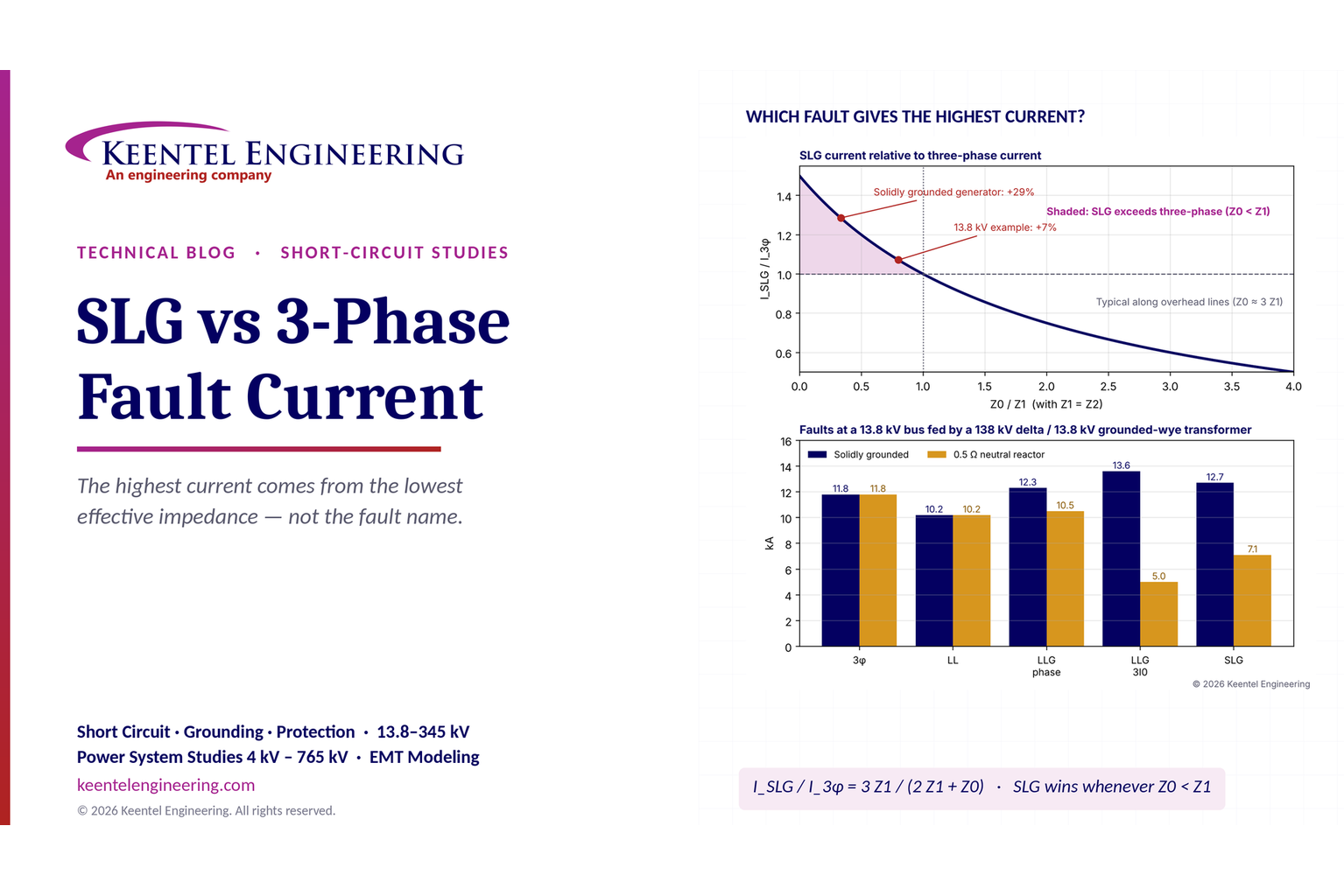
Learn which fault produces the highest current at a bus, why SLG faults can exceed three-phase faults, and how symmetrical components determine fault duty.
By SANDIP R PATEL
•
October 11, 2026
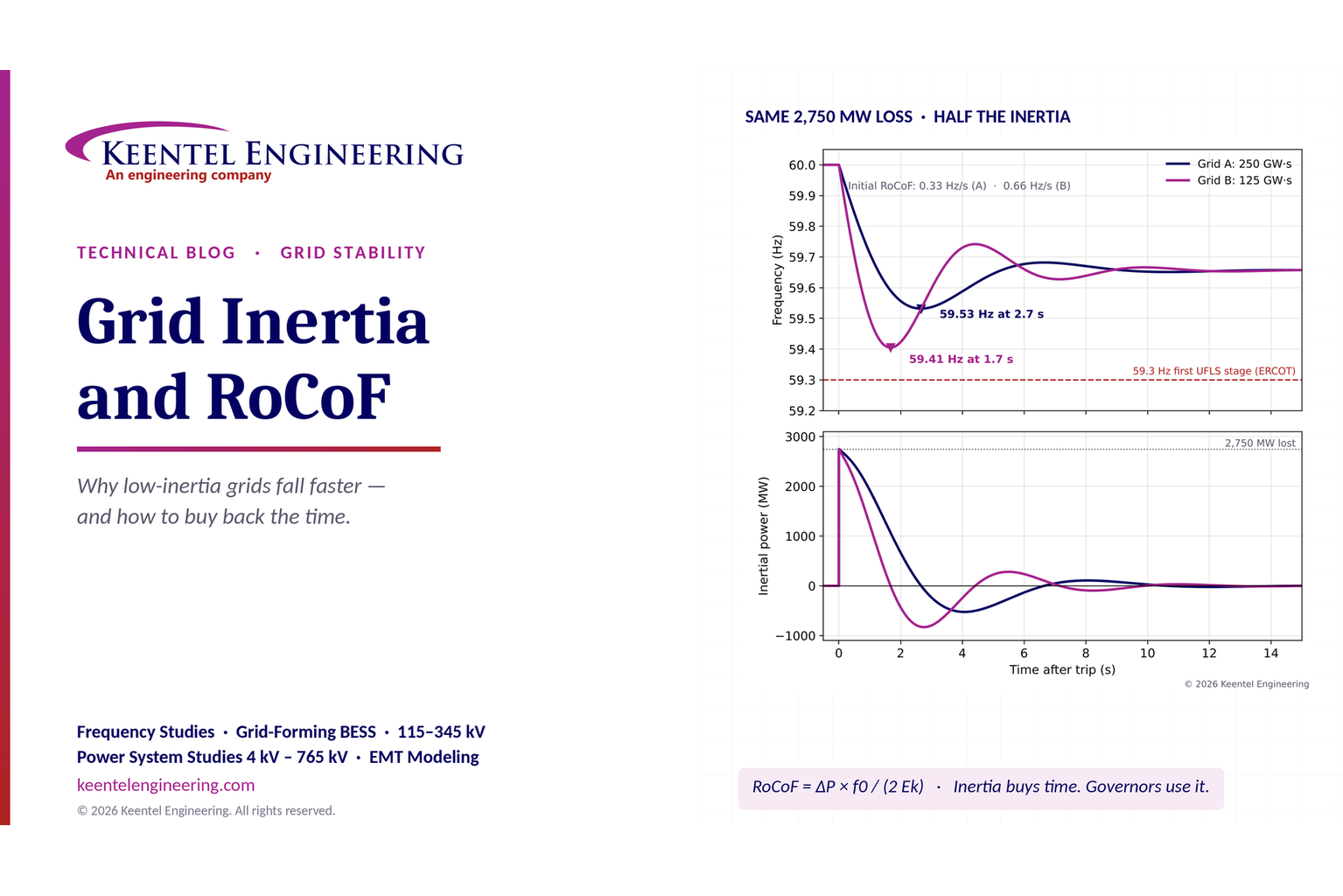
Explore grid inertia, RoCoF and frequency response, with swing equation calculations, frequency nadir analysis and US power system simulation examples.
By SANDIP R PATEL
•
October 11, 2026
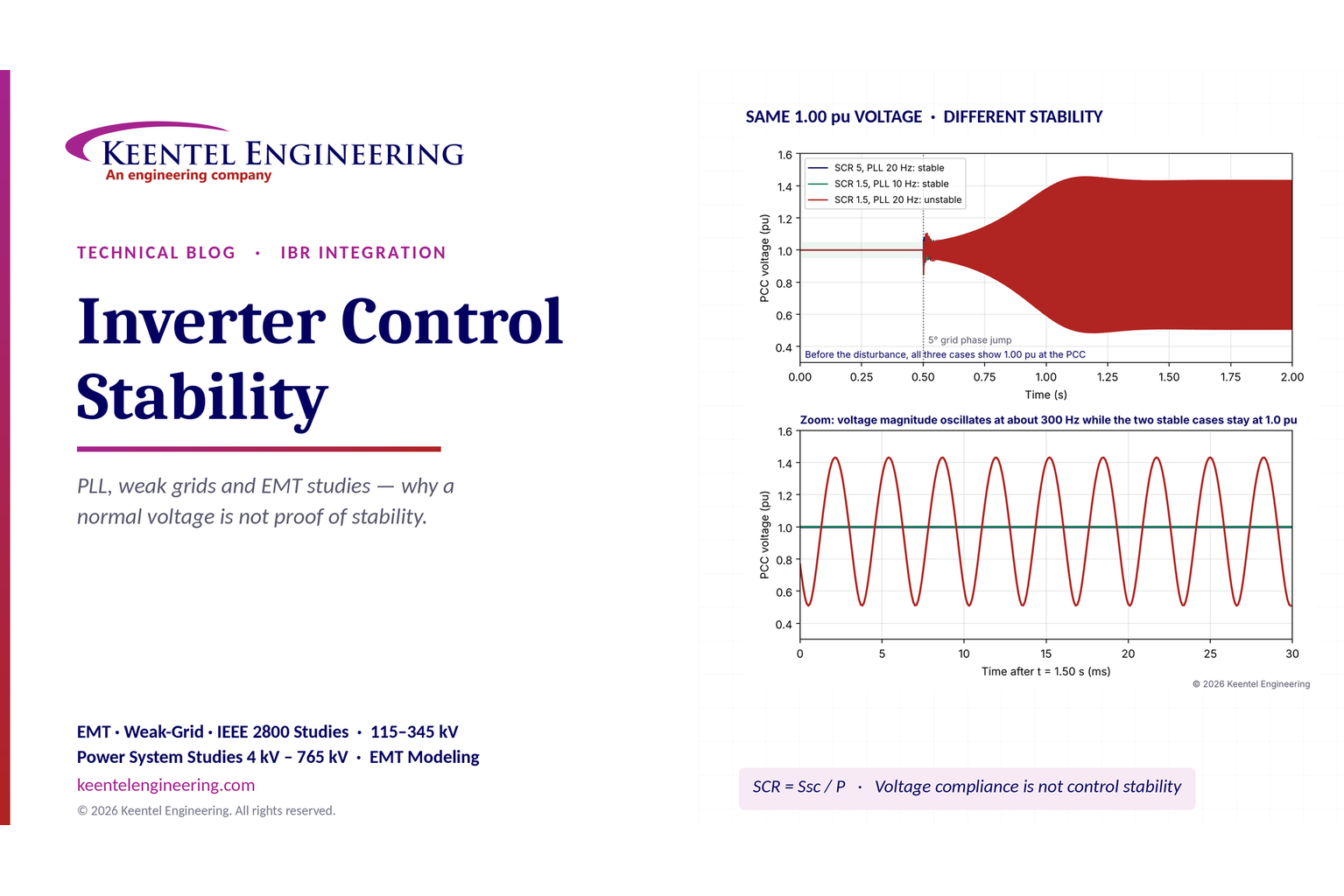
Learn why inverter controls become unstable in weak grids, how PLL bandwidth and SCR affect stability, and how PSCAD EMT studies identify and mitigate oscillations.
By SANDIP R PATEL
•
October 11, 2026
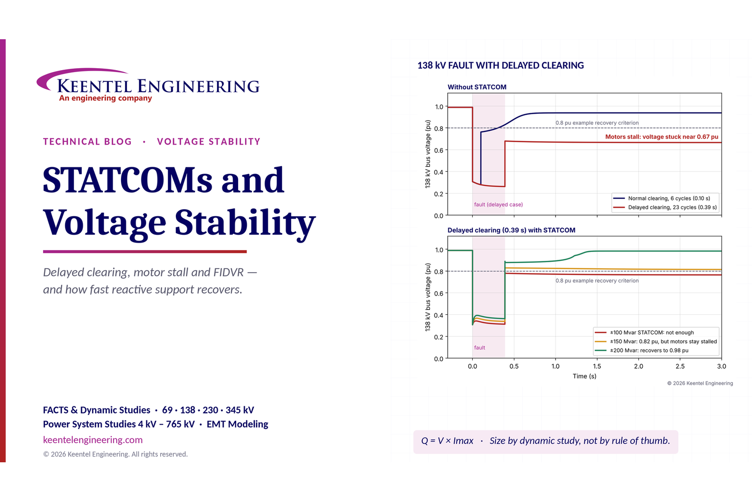
Learn how STATCOMs improve voltage stability and prevent FIDVR. Explore reactive power sizing, delayed fault clearing, NERC criteria and 138 kV simulation results.
By SANDIP R PATEL
•
October 10, 2026
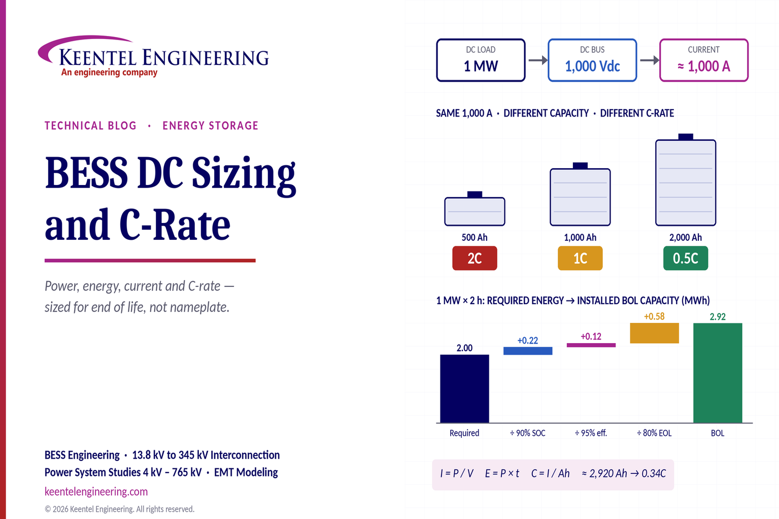
Learn BESS DC sizing with power, energy, current and C-rate calculations, battery losses, degradation and a 100 MW/400 MWh utility-scale example.
By SANDIP R PATEL
•
October 10, 2026
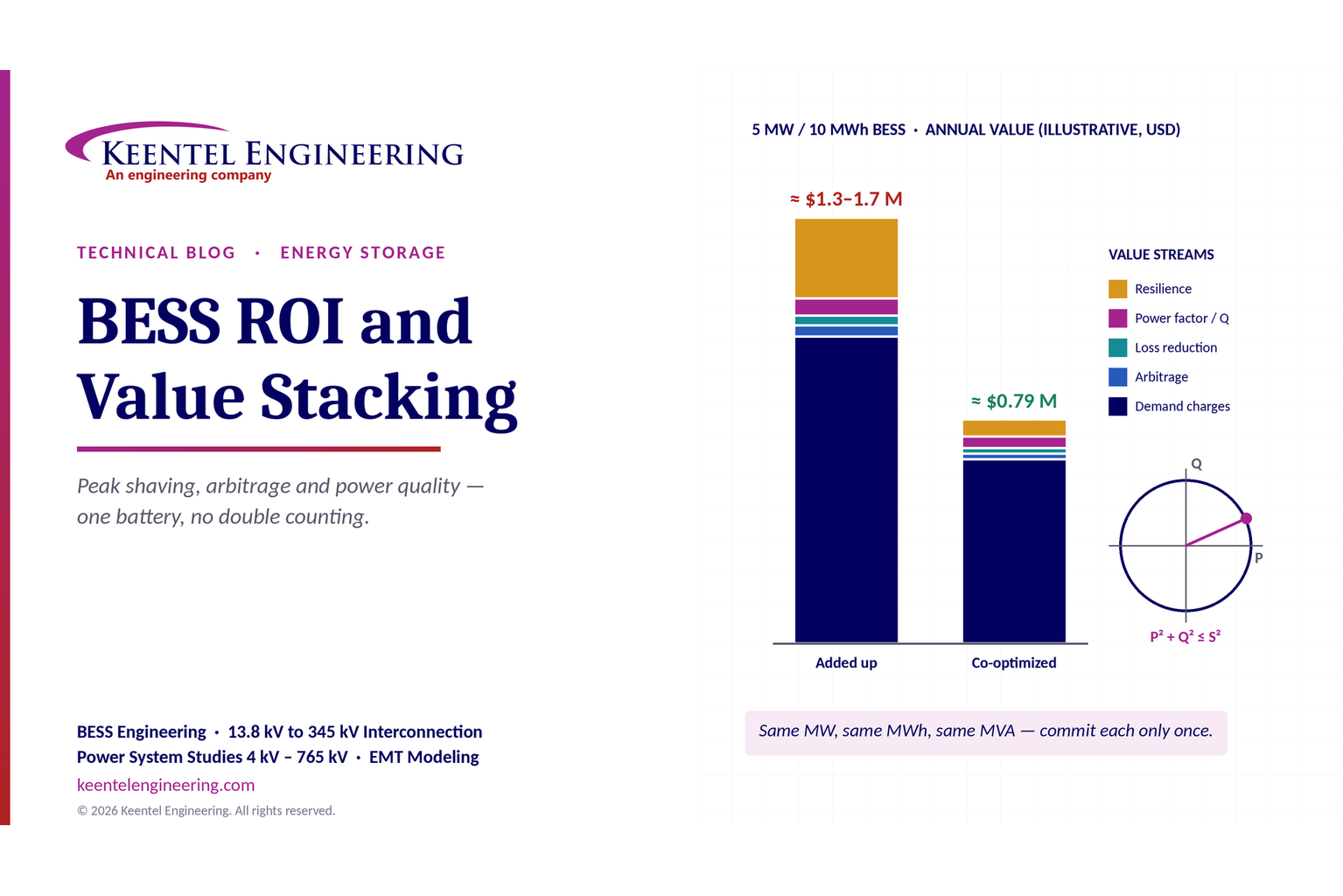
Learn how BESS ROI is calculated using peak shaving, energy arbitrage, power quality and battery storage economics, with a practical 5 MW/10 MWh example.
By SANDIP R PATEL
•
October 10, 2026
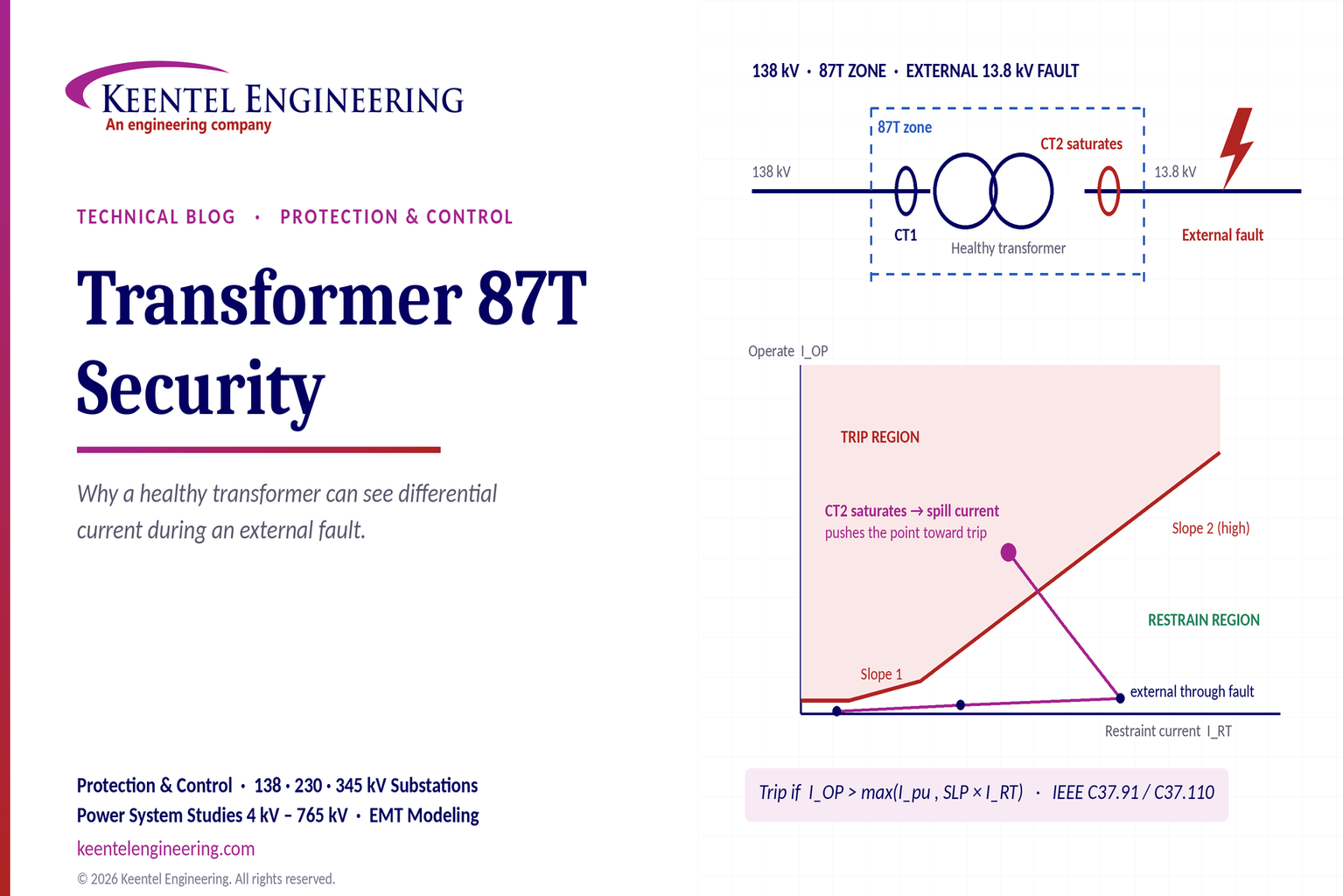
Learn why transformer differential relays detect current during external faults, how CT saturation causes spill current, and how secure 87T protection prevents trips.
By SANDIP R PATEL
•
October 10, 2026
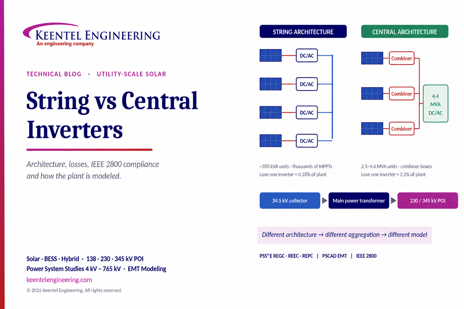
Compare string vs central inverters for utility-scale solar, including efficiency, maintenance, grid compliance, reactive power and interconnection studies.
By SANDIP R PATEL
•
October 9, 2026
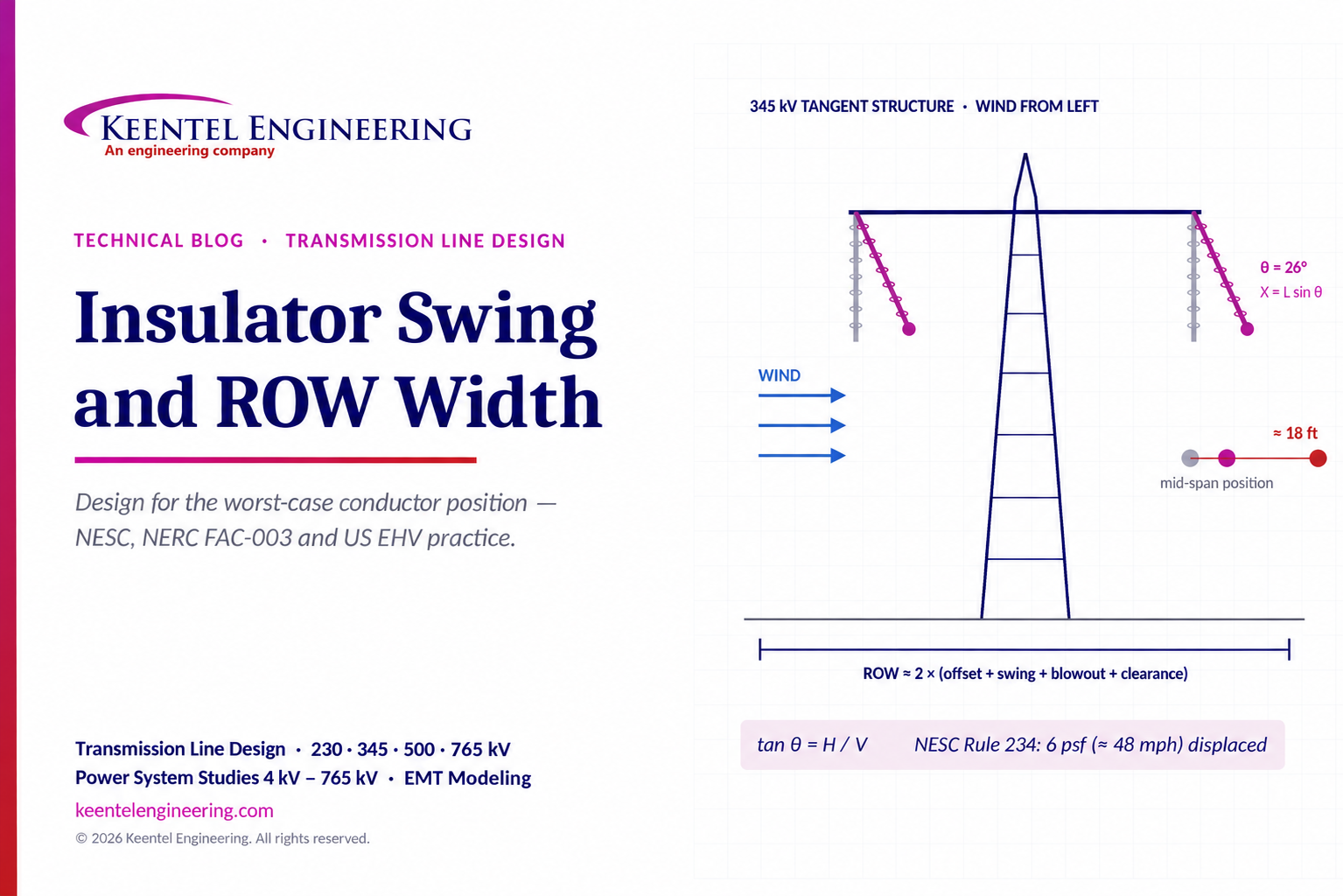
Learn how insulator swing angle and conductor blowout affect transmission line ROW width, with NESC clearances, NERC FAC-003 guidance, and a 345 kV example.
Copy